Architecting a Game Loop in C#: Building a Real-Time Simulation Engine Step by Step

1 The Philosophy of Time: Simulations vs. Reactive Systems

Real-time simulation engines live in a different world from typical business applications. They don’t respond to a request and return a result—they create time. A simulation engine is responsible for advancing the world forward in consistent, measurable steps, even if no one is watching. That difference shapes everything about how we architect the loop, model time, handle precision, and manage computing resources.

When I walk senior engineers through this paradigm shift, I often compare it to running an entire operating system inside your application. You own the clock. You determine what “now” means. And you decide how the state evolves every tick. Understanding this philosophy of time is the foundation for building a robust C# game loop or real-time simulation engine that behaves predictably under load.

1.1 Beyond Request/Response

Traditional .NET services—web APIs, background workers, message processors—live in a reactive environment. Something external wakes them. A user hits a URL, a queue pushes a message, or a scheduled job fires. Each execution is isolated. Time isn’t continuous; it’s chopped into discrete requests.

A simulation engine follows a completely different rhythm. It must run continuously in its own world and advance its state whether or not inputs are arriving. This is what makes a simulation loop fundamentally different from event-driven architectures.

1.1.1 Event-Driven Architecture vs. Simulation Architecture

Take an example: an ASP.NET Core API that calculates pricing for a basket of equities. Every request is independent. You run the math, return a result, and go idle. The runtime, the OS, the scheduler—they decide when your code runs again.

Now imagine you’re building a real-time financial engine computing risk metrics 60 times per second. Or a robotics controller adjusting servo positions in tight feedback loops. Or a game engine updating physics and AI every 16.666 milliseconds.

Here, you cannot wait for a request. You run continuously, and the world must advance at a fixed pace. If a player pauses or an input is missing, the world must continue making progress. The simulation owns time itself.

1.1.2 Why await Task.Delay() and Standard Timers Don’t Work

I see this mistake constantly:

while (true)
{
    UpdateWorld();
    await Task.Delay(16); // ~60 fps?
}

It looks clean. It’s wrong.

Timers and Task.Delay() depend on OS scheduling and internal timer resolution. On Windows, timer resolution often defaults to 15.6 ms, which means you can’t reliably produce a 16.666 ms cadence. A 1–2 ms deviation might seem small, but it accumulates into jitter, instability, and nondeterminism.

Even modern .NET timers—PeriodicTimer, System.Threading.Timer—depend on OS-level tick granularity. They can drift. They can bunch. They can fire late under CPU load. None of this works when you need hard, predictable cadence.

A real simulation engine needs something closer to a heartbeat—a consistent pulse tied to real clock time but driven manually.

1.1.3 The Heartbeat of the System

The game loop or simulation loop acts as the system’s heartbeat. Each beat advances everything: physics, AI, market data, sensor fusion, etc. If the heartbeat becomes irregular, the world becomes unstable.

This heartbeat is explicitly controlled:

• You read clock time.
• You compute elapsed time.
• You advance simulation time in small, deterministic increments.
• You correct for drift each cycle—not depend on a timer to “be accurate.”

This is why the loop is the architecture. Everything else builds on how you measure, advance, and interpret time.

1.2 The Trinity of Real-Time Systems

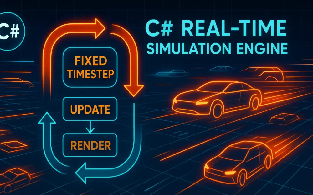
Most real-time systems—games, robotics platforms, trading engines—follow the same three-phase loop. The names vary, but the pattern is universal.

1.2.1 Input Phase: External Signals

Inputs enter the simulation from the outside world. They can arrive at arbitrary times and must be incorporated into the next update phase cleanly. In real-time engines, we treat inputs as events queued for the next tick.

Examples:

• Keyboard or controller input
• Touchscreen gestures
• Market orders or sensor packets
• Network replication data from clients

Because the simulation loop is authoritative, inputs don’t directly mutate the state. They merely request changes. The loop decides how to integrate them.

1.2.2 Update Phase: Advancing the World State

This is the heart of the simulation. Everything that exists in the world is advanced mathematically using a fixed time step, such as 1/60th of a second.

This is where:

• Vehicle velocities integrate into new positions
• Physics forces resolve
• Financial instruments accrue interest or risk metrics
• NPCs evaluate decision trees
• Projectiles move on trajectories

What matters is consistency. Every update step must represent the same duration of simulated time, even if wall-clock time varies due to hardware or OS load.

1.2.3 Render Phase: Presenting the State

Render does not change the world. It merely reads from it.

Rendering may occur at different frequencies:

• Graphics engines may render at 144 Hz or 240 Hz.
• Server engines may broadcast snapshots at 20–30 Hz.
• Sensor systems may stream processed data at a rate the downstream devices can handle.

That difference is why we often decouple rendering from updating. As long as the simulation produces stable states at a predictable frequency, the presentation layer can interpolate between states to smooth things out.

1.3 The Determinism Challenge

If you run your simulation twice on two different machines, do you get the same answer? In a real-time engine, that question is foundational.

1.3.1 Defining Determinism

A deterministic simulation produces the same outputs when given the same inputs, regardless of:

• CPU model
• Thread scheduling
• Instruction timing
• Clock drift
• Floating-point behavior

This sounds simple. It isn’t.

1.3.2 Floating-Point Precision Issues

Floating-point arithmetic is not associative:

(a + b) + c != a + (b + c)

Two cores may compute the same expression in different orders. GPUs and SIMD instructions can produce different rounding results. Cross-platform differences (x86 vs. ARM) matter. Even compiler optimizations affect results.

A small rounding difference in a physics simulation can cause objects to collide earlier on one machine than another, changing the entire world state from that point forward.

1.3.3 Race Conditions in Simulation

A classic nondeterminism trap:

Parallel.ForEach(entities, e => e.Update());

If the simulation depends on update ordering, parallelism introduces randomness. One race condition may appear once in a million ticks but cause catastrophic divergence.

Financial simulations suffer similarly. Suppose an engine processes interest accrual in a non-deterministic order; two servers replicating the same market will diverge.

Determinism requires strict ordering, strict time advancement, and careful numerical approaches.

---

2 The “Broken” Loop: Analyzing Naive Implementations

Before building the correct loop, we examine what goes wrong in typical C# implementations. Most developers start with something simple—and that simplicity hides pathological behavior under load.

2.1 The “While(True)” Trap

Developers often attempt the simplest infinite loop:

while (true)
{
    Update();
}

This loop saturates a CPU core immediately. It spins at 100% utilization, consuming every available cycle. And because nothing yields or sleeps:

• The OS scheduler may throttle the thread.
• CPU Boost frequencies fluctuate.
• Other processes starve.
• Power consumption spikes.
• Thermal throttling kicks in.

All of these influence timing unpredictably.

2.1.1 Why CPU Throttling Breaks Simulation Timing

Modern CPUs dynamically adjust performance:

• Boost high for burst work
• Reduce clocks under sustained load
• Throttle under thermal pressure

A loop that runs “as fast as it can” today might run at 5%–10% lower speed after 30 seconds of heat buildup. If your algorithm uses actual wall-clock delta time to compute physics, everything slows down.

2.1.2 OS Scheduler Slicing

Even a dedicated thread is not truly dedicated. Windows, Linux, and macOS may preempt your thread at any time. When a context switch occurs, your loop stalls for a few hundred microseconds. That jitter destroys timing precision.

Incorrect approach:

var last = DateTime.UtcNow;

while (true)
{
    var now = DateTime.UtcNow;
    var dt = now - last;
    last = now;

    Update(dt.TotalSeconds); // unstable delta
}

DateTime.UtcNow has coarse resolution (0.5–1 ms). Scheduler jitter adds noise. Over minutes, drift becomes visible. Over hours, the simulation becomes inconsistent.

2.2 Variable Time Step (Delta Time) Issues

Using variable delta time seems natural. You compute how much time has passed since the last frame and use it directly.

The problem is instability. Variable time steps lead to unpredictable motion, collision issues, and divergent simulation results.

2.2.1 Tunneling Effect Example

Consider a projectile moving at 10 units per frame. If the delta time spikes, say from 16 ms to 50 ms, the projectile may “jump” past a thin wall entirely without collision detection.

This is common in physics engines and is the reason fixed time stepping is considered the gold standard.

2.2.2 Financial Case Study: Inconsistent Interest Compounding

Imagine computing compound interest in a trading engine:

balance += balance * (rate * dt)

If dt varies:

• Fast machines accrue interest more frequently and get more compounding.
• Slower machines accrue less frequently and get different results.

Over thousands of ticks, values diverge significantly.

A trading engine must be deterministic, or reconciliation becomes impossible.

2.3 The Spiral of Death

This is the infamous feedback loop all real-time developers encounter:

1. One update takes slightly too long.
2. The delta time becomes larger next tick.
3. A larger dt means more simulation work.
4. Which increases the tick time again.
5. And so on…

Eventually, the engine cannot recover. Frame rate collapses. Simulation time drifts catastrophically.

2.3.1 Corrective Measures: Clamping dt

The standard defense is to clamp delta time:

var dt = Math.Min(elapsed, maxStep);

This ensures that even if the simulation lags for a moment, it only advances a small, predictable amount of time each tick.

It avoids spirals but doesn’t fix the fundamental problem of variable time stepping.

---

3 Architecting the Canonical Loop: Fixed Time Steps

This is the architecture used by most real-time engines: Unity, Godot, Unreal (for physics), robotics simulators, and serious financial models. The idea is simple:

Always advance simulation time in equal increments, regardless of how long each update takes in real time.

3.1 The “Fix Your Timestep” Pattern

First formalized by Glenn Fiedler, the “Fix Your Timestep” model introduced the accumulator pattern, which separates wall-clock time from simulation time.

3.1.1 Decoupling Wall Clock vs. Simulation Time

We measure real elapsed time (wall clock). But we don’t feed that directly into physics.

Instead:

• Accumulate elapsed time in a buffer.
• Consume fixed-size chunks (like 16.666 ms).
• Run Update() once per chunk.
• Carry leftover time to the next loop.

This keeps simulation time perfectly stable even when real time fluctuates slightly.

3.1.2 Accumulator Loop in C#

Here is a production-ready core loop using Stopwatch:

public class SimulationLoop
{
    private readonly TimeSpan _fixedTimeStep = TimeSpan.FromTicks(166666); // 60 Hz, exact
    private readonly Stopwatch _stopwatch = new();

    public void Run()
    {
        _stopwatch.Start();
         var accumulator = TimeSpan.Zero;
        var previous = _stopwatch.Elapsed;
       
        while (true)
        {
            var now = _stopwatch.Elapsed;
            var frameTime = now - previous;
            previous = now;

            accumulator += frameTime;

            while (accumulator >= _fixedTimeStep)
            {
                Update(_fixedTimeStep);
                accumulator -= _fixedTimeStep;
            }

            // 'alpha' is the interpolation fraction between previous and current simulation states
            Render(accumulator / _fixedTimeStep);
        }
    }
    private void Update(TimeSpan dt)
    {
        // Advance the deterministic world state by a fixed time step (dt)
    }
    
    /// <summary>
    /// Interpolates between simulation states using the alpha value to provide smoother presentation during rendering.
    /// </summary>
    private void Render(double alpha)
    {
        // Interpolate using alpha
    }
    
}

3.1.3 Why This Works

• Slow frames cause multiple simulation steps, keeping time consistent.
• Fast frames may perform zero updates but will still render.
• The accumulator ensures we neither fall behind nor race ahead.
• The simulation always advances in fixed increments.
• Rendering can be smoother than simulation through interpolation.

This is the gold standard.

3.2 Handling Residual Time

After consuming as many full steps as possible, a small amount of leftover time remains. That residual creates the interpolation alpha.

3.2.1 Substep Fraction (alpha)

alpha = accumulator / fixedStep

This value is between 0 and 1. It tells you how far into the next simulation step you are. Rendering uses this to interpolate between PreviousState and CurrentState.

3.2.2 Why Residual Time Improves Smoothness

Without interpolation, rendering looks jittery because the simulation updates discretely. Interpolation allows the renderer to produce smooth motion even when the update rate is lower than the refresh rate.

Residual time is not used for physics or state mutation; it’s only used for presentation.

3.3 Modern .NET Timing Mechanisms

.NET provides several time APIs, but only a few are suitable for precise loop control.

3.3.1 Stopwatch vs. DateTime.UtcNow

DateTime.UtcNow:

• Resolution ~0.5–1 ms on Windows.
• Affected by system time adjustments.
• Too coarse for simulation timing.

Stopwatch:

• High-resolution (microseconds or better).
• Monotonic (never moves backward).
• Based on QueryPerformanceCounter on Windows.

Always use Stopwatch.

3.3.2 Is PeriodicTimer (NET 6+) Good for Loops?

PeriodicTimer is great for:

• Background tasks
• Consistent scheduling with reasonable tolerance

However, it’s not ideal for simulation loops:

• Depends on OS timer resolution.
• Jitter can be 1+ ms.
• Cannot guarantee stable cadence at 60+ Hz.
• Not suitable for determinism.

It works fine for:

• Telemetry batching
• Low-frequency logic (5–20 Hz)
• Non-critical background subsystems

But not for core simulation timing.

3.3.3 High-Resolution Ticks with Stopwatch.GetTimestamp()

For very high-frequency loops or nanosecond-level math, use raw timestamp values:

long ticks = Stopwatch.GetTimestamp();
double seconds = ticks / (double)Stopwatch.Frequency;

This gives:

• Sub-microsecond precision
• Stable timing on all supported platforms
• No system clock interference

Many physics engines convert everything to integer tick math for determinism.

---

4 State Interpolation and Decoupling Presentation

Up to this point, we have a stable fixed-step simulation loop that advances world state deterministically. What usually comes next is the realization that the simulation and the presentation layers rarely operate at the same rate. Your simulation might run at 60 updates per second, but your rendering or broadcast layer could run much faster—or much slower. When those rhythms don’t align, visual jitter, stutter, and inconsistencies appear. This is where interpolation and decoupling become essential architectural tools.

4.1 The Visual Jitter Problem

A common scenario in modern systems is mismatched frequencies: a simulation at 60 Hz and a GPU running at 144 Hz, or a server broadcasting snapshots at 20 Hz while clients render at 120 Hz. Because the simulation only produces discrete states at fixed intervals, the renderer must fill the gaps. If the renderer draws using only the “current” simulation frame, it will repeatedly show the same state until the next update arrives. When the simulation advances, the renderer suddenly jumps to the next state. Those jumps appear as jitter.

For developers building authoritative servers, it’s easy to forget that visualization can be just as sensitive to timing abnormalities as physics. Even console-based dashboards or telemetry panels suffer from jitter when consuming state updates slower than their presentation loop. Every time the renderer exposes a discontinuity between consecutive frames, the user notices lag, jerkiness, or discontinuous motion. Interpolation is what smooths these transitions.

Another source of jitter appears when rendering outpaces the simulation. If the screen refreshes 240 times per second but the simulation only produces a new state every 16.666 ms, the renderer spends most frames redrawing stale data. Without interpolation, motion feels uneven because the simulation produces “chunks” of movement rather than smooth arcs. Bridging those chunks with interpolation keeps motion coherent.

4.2 Implementing Linear Interpolation (Lerp)

The simplest form of interpolation for real-time systems is linear interpolation (“lerp”). We blend between two known simulation states using an alpha that represents how far we are between the last update and the next one. The simulation loop already computes this value indirectly through the accumulator’s leftover time.

4.2.1 Using Residual Time to Compute Alpha

From the accumulator logic, alpha is:

alpha = accumulator / fixedTimeStep

This ratio is guaranteed to be between 0 and 1. It represents how far the renderer is into the next expected simulation step. If alpha is closer to 0, we are close to the previous state; if it’s closer to 1, we are close to the next state.

The general formula is:

State_render = State_previous * (1 - alpha) + State_current * alpha

This works for positions, rotations (with special handling), prices, and most scalar or vector values that evolve predictably.

4.2.2 Example: Interpolating an Entity’s Position

Here is a straightforward interpolation example using a simple state struct:

public readonly struct EntityState
{
    public readonly Vector2 Position;
    public readonly float Rotation;

    public EntityState(Vector2 pos, float rot)
    {
        Position = pos;
        Rotation = rot;
    }
}

public static class Interpolator
{
    public static EntityState Interpolate(in EntityState previous, in EntityState current, double alpha)
    {
        var pos = Vector2.Lerp(previous.Position, current.Position, (float)alpha);
        var rot = previous.Rotation + (float)alpha * (current.Rotation - previous.Rotation);
        return new EntityState(pos, rot);
    }
}

This code mirrors what the renderer needs: two stable snapshots and a blend factor. Since interpolation is read-only and stateless, it slots neatly into the render loop without interfering with the simulation. The tricky part isn’t the math—it’s managing the data safely.

4.3 The Double-Buffer State Pattern

With interpolation, the renderer needs both “previous” and “current” simulation states. That means the simulation thread must produce stable snapshots at the end of each tick. If the renderer reads state while the simulation is mutating it, nondeterminism and tearing occur. The cleanest solution is a double-buffer pattern.

4.3.1 Maintaining Two Buffers

You maintain two buffers:

• PreviousState
• CurrentState

When the simulation finishes a tick:

1. Copy CurrentState into PreviousState.
2. Write the updated world state into CurrentState.

Neither buffer is ever mutated after this point in the tick. On the rendering side, interpolation only reads from these buffers, ensuring consistency.

4.3.2 Example: Double-Buffered Snapshot Container

Below is a simple pattern for double-buffering:

public class StateBuffer<T> where T : struct
{
    private T _previous;
    private T _current;

    public void SwapAndSetCurrent(in T newState)
    {
        _previous = _current;
        _current = newState;
    }

    public void GetStates(out T previous, out T current)
    {
        previous = _previous;
        current = _current;
    }
}

This approach eliminates the need for locks during rendering because state mutations occur predictably once per tick. In high-frequency systems, removing locks from the hot path is critical. By structuring the simulation around clear, atomic state transitions, you make interpolation safe and efficient.

---

5 Advanced Concurrency: The Multi-Threaded Loop

At some point, simulation and rendering compete for time on the same thread. Physics, AI, pathfinding, or financial models may consume too much CPU time, leaving little room for rendering or broadcasting. The natural next step is splitting them into separate threads. This isn’t trivial, but it’s one of the highest-impact architectural changes you can make.

5.1 Breaking the Single-Threaded Paradigm

In a single-threaded loop, simulation and presentation occur in sequence. If the simulation stalls for a few milliseconds, rendering stalls too. That tension becomes more pronounced as systems scale. Moving rendering or broadcasting to another thread frees the simulation to run as fast and consistently as needed.

The simulation thread keeps strict determinism: fixed steps, consistent tick progression, state snapshots. The rendering or broadcasting thread consumes those snapshots at its own pace. This division allows each subsystem to run at optimal frequencies and reduces jitter from long-running updates.

Even simple servers benefit from this split. A trading engine, for example, might compute risk metrics at 60 Hz while a network thread pushes updates to clients at 20 Hz. Decoupling those responsibilities keeps the simulation clean and predictable.

5.2 Producer-Consumer Architecture with System.Threading.Channels

When splitting threads, you need a safe, low-latency way to transfer data between them. System.Threading.Channels is one of the best tools in .NET for this. Channels model a producer-consumer pattern with bounded or unbounded capacity. For simulation loops, bounded channels are ideal.

5.2.1 Producing Snapshots

Each tick, the simulation thread produces a snapshot. Instead of handing it directly to the renderer, you push it into a channel.

var channel = Channel.CreateBounded<EntityState>(new BoundedChannelOptions(4)
{
    SingleWriter = true,
    SingleReader = true,
    FullMode = BoundedChannelFullMode.DropOldest
});

Setting DropOldest means the channel discards stale frames rather than blocking the simulation. This is important: the simulation must never wait on the renderer.

Producing a snapshot:

await channel.Writer.WriteAsync(currentState);

Because the simulation must remain deterministic and time-bound, it writes once per tick, no matter what.

5.2.2 Consuming Snapshots

The rendering thread reads as fast as it can:

await foreach (var state in channel.Reader.ReadAllAsync())
{
    RenderState(state);
}

The renderer always consumes the latest state available. If the renderer is slower than the simulation, it silently drops older states. This keeps both systems behaving optimally without blocking each other.

5.2.3 Handling Backpressure

There are three common strategies:

1. DropOldest – Best for rendering; ensures the most recent frame is rendered.
2. DropNewest – Occasionally useful in data streams where older frames matter more.
3. Wait – Never use this for simulations; waiting breaks cadence.

Choosing the right backpressure strategy ensures system stability without breaking determinism.

5.3 Thread Safety and Synchronization

The biggest mistake I see is using too many locks. Locks in a simulation loop introduce jitter, create contention, and occasionally deadlock under corner cases. The simulation thread’s hot path must avoid locks entirely.

5.3.1 Avoiding Contention

Instead of locking around shared data, design your architecture so the simulation never shares mutable state directly with other threads. Channels, double buffers, and immutable snapshots all prevent the need for locks.

5.3.2 Using Interlocked and Memory Barriers

Sometimes you need flags or state indicators. These must be atomic. Here’s an example of a simple shutdown flag:

private int _shutdownRequested = 0;

public void RequestShutdown()
{
    Interlocked.Exchange(ref _shutdownRequested, 1);
}

private bool IsShutdownRequested => Volatile.Read(ref _shutdownRequested) == 1;

Interlocked ensures writes are atomic. Volatile.Read creates a memory barrier ensuring the simulation thread sees updates promptly. This pattern is lightweight and suitable for high-frequency loops.

---

6 Data Structures and Memory Management (Data-Oriented Design)

Real-time simulation loops stress memory and CPU in unusual ways. Iterating through thousands of entities every tick multiplies even minor inefficiencies into measurable slowdowns. Data-oriented design puts memory layout first, not object relationships, because the CPU spends more time waiting for memory than computing math.

6.1 The Cost of Garbage Collection (GC) in Loops

GC pauses—even short ones—break determinism and timing stability. Any allocation inside your Update() loop is a potential latency spike waiting to happen. The most common hidden allocations include:

• Lambda captures and closures
• LINQ operators
• Boxing in generic collections
• String concatenation
• Implicit array resizing
• Deferred-execution enumerators

Even a seemingly harmless LINQ statement can allocate dozens of objects. The fix is straightforward: avoid new in the loop and eliminate features that generate hidden allocations.

6.1.1 Example of Hidden Allocation (Incorrect)

foreach (var e in entities.Where(x => x.IsActive))
{
    e.Update();
}

This allocates an iterator plus intermediate state.

6.1.2 Corrected Version

for (int i = 0; i < entities.Count; i++)
{
    ref var e = ref entities[i];
    if (e.IsActive)
        e.Update();
}

This version avoids allocations, uses references where possible, and improves cache locality.

6.2 Structs vs. Classes for State

Structs shine in simulation engines because they can be stored contiguously in memory, leading to efficient iteration. Classes scatter objects around the heap, creating cache misses.

6.2.1 Using ref struct and readonly struct

ref struct ensures stack-only storage, ideal for temporary data used within a single tick. readonly struct guarantees immutability and encourages the compiler to optimize field access.

Example:

public readonly struct VehicleState
{
    public readonly Vector2 Position;
    public readonly Vector2 Velocity;

    public VehicleState(Vector2 p, Vector2 v)
    {
        Position = p;
        Velocity = v;
    }
}

Since the state is compact and immutable, iterating over thousands of instances becomes predictable and cache-friendly.

6.2.2 Understanding Cache Lines

Modern CPUs load memory in chunks called cache lines (typically 64 bytes). If your entities are packed in arrays, scanning them is extremely fast. But if they’re scattered across the heap, you incur cache misses, forcing the CPU to stall while pulling data from RAM.

Data-oriented design aligns memory layout with iteration patterns, drastically improving throughput.

6.3 Entity Component System (ECS) Basics

ECS architectures restructure data around three core ideas:

1. Entities are simple identifiers.
2. Components are struct-like data.
3. Systems operate on contiguous arrays of components.

For simulation-heavy workloads, ECS is often the most performant approach because each system touches only the data it needs, and related data lives together in memory.

6.3.1 Choosing an ECS Library

Two popular C# ECS frameworks worth considering:

• Arch – Lightweight, high-performance ECS with a clean API.
• Svelto.ECS – More opinionated but excellent for large-scale simulations.

Both libraries prioritize memory layout and deterministic iteration order. Rolling your own ECS can work, but maintaining it becomes a cost in itself.

6.3.2 Example: Simple Array-Based Manager

Here’s a minimal manager that embraces data locality:

public class VehicleManager
{
    public VehicleState[] States;

    public VehicleManager(int count)
    {
        States = new VehicleState[count];
    }

    public void UpdateAll(in TimeSpan dt)
    {
        for (int i = 0; i < States.Length; i++)
        {
            ref var state = ref States[i];
            var newPos = state.Position + state.Velocity * (float)dt.TotalSeconds;
            States[i] = new VehicleState(newPos, state.Velocity);
        }
    }
}

The contiguous array minimizes cache misses during sequential updates.

6.4 Object Pooling

For systems that go beyond pure struct storage—spawning temporary objects, allocating buffers, or handling network packets—object pooling is crucial. Pooling amortizes allocation cost and prevents GC churn.

6.4.1 Using Microsoft.Extensions.ObjectPool

Microsoft’s object pooling library provides reusable pools with configurable policies.

public class EntityPoolPolicy : IPooledObjectPolicy<Entity>
{
    public Entity Create() => new Entity();
    public bool Return(Entity obj)
    {
        obj.Reset();
        return true;
    }
}

var provider = new DefaultObjectPoolProvider();
var pool = provider.Create(new EntityPoolPolicy());

Instead of calling new Entity() repeatedly inside the simulation, you request and return items from the pool.

6.4.2 Custom Pool Example

If you need manual control:

public class SimplePool<T> where T : class, new()
{
    private readonly Stack<T> _stack = new();

    public T Rent() => _stack.Count > 0 ? _stack.Pop() : new T();

    public void Return(T obj) => _stack.Push(obj);
}

This pool is simplistic but effective for internal systems where you control lifecycle tightly.

---

7 Practical Implementation: The “LogiSim” Traffic Engine

To bring all the earlier architectural concepts together, we’ll build a practical real-time simulation: LogiSim, a simplified traffic engine responsible for simulating 10,000 autonomous vehicles moving across a 2D grid. The goal isn’t to build a photorealistic renderer or a full physics engine—it’s to show how the fixed-step loop, interpolation, data-oriented design, and concurrency patterns work together in a real system. This example mirrors what I’ve built for robotics, logistics, and traffic-flow research, where determinism and performance matter more than visual fidelity.

7.1 Defining the Requirements

The LogiSim engine must simulate a dense grid containing thousands of vehicles. Each vehicle updates its position and velocity every tick. The simulation infrastructure must run at exactly 60 UPS, regardless of machine speed. Deterministic progression matters because different instances of the engine may validate each other’s results, a common requirement in distributed robotics and market simulation environments.

The traffic model is intentionally simple. Vehicles have a position and velocity and avoid collisions by sampling nearby cells. Real-world traffic simulators use far more complex behavioral models, but those would distract from the architecture itself. Our focus is on throughput, clarity, and deterministic progression—each tick should take the same amount of simulated time, and all state transitions must be reproducible.

Finally, we must maintain smooth presentation. The simulation thread will produce state snapshots at 60 Hz, while a lightweight renderer consumes snapshots and interpolates between them. The mismatch between simulation and presentation rates is exactly why interpolation and multi-threading matter.

7.2 Building the Core

Before wiring rendering or shifting work to multiple threads, we focus on the foundation: the simulation loop and the state buffers. These form the stable core that everything else depends on. We reuse the fixed-step accumulator architecture introduced earlier and adapt it specifically for LogiSim.

7.2.1 The VehicleState Struct

Each vehicle tracks only position and velocity. Using Vector2 keeps the struct small and efficient.

public readonly struct VehicleState
{
    public readonly Vector2 Position;
    public readonly Vector2 Velocity;

    public VehicleState(Vector2 position, Vector2 velocity)
    {
        Position = position;
        Velocity = velocity;
    }

    public VehicleState Integrate(float dt)
    {
        var newPos = Position + Velocity * dt;
        return new VehicleState(newPos, Velocity);
    }
}

Integrate makes deterministic updates easy to reason about and inlines well during compilation. This helps in loops touching thousands of vehicles.

7.2.2 The SimulationLoop for LogiSim

The simulation loop follows the fixed-step accumulator design. Instead of using placeholder methods, we bind real update logic and snapshot production.

public class LogiSimLoop
{
    private readonly TimeSpan _step = TimeSpan.FromTicks(166666); // 60 Hz, exact
    private readonly Stopwatch _sw = new();
    private readonly VehicleManager _manager;
    private readonly Channel<VehicleState[]> _snapshotChannel;

    public LogiSimLoop(VehicleManager manager, Channel<VehicleState[]> snapshotChannel)
    {
        _manager = manager;
        _snapshotChannel = snapshotChannel;
    }

    public void Run()
    {
        _sw.Start();
        var previous = _sw.Elapsed;
        var accumulator = TimeSpan.Zero;

        while (true)
        {
            var now = _sw.Elapsed;
            var frame = now - previous;
            previous = now;

            accumulator += frame;

            while (accumulator >= _step)
            {
                _manager.UpdateAll(_step);
                accumulator -= _step;

                // produce snapshot for renderer
                var snapshot = _manager.CloneStates();
                _snapshotChannel.Writer.TryWrite(snapshot);
            }

            Thread.Yield();
        }
    }
}

This loop guarantees 60 updates per second of simulation time. The render thread uses the channel to acquire snapshots and interpolate them.

7.2.3 The VehicleManager Storage

The manager stores vehicle states using contiguous arrays for cache locality.

public class VehicleManager
{
    private VehicleState[] _states;

    public VehicleManager(int count)
    {
        _states = new VehicleState[count];
        var random = new Random(42);

        for (int i = 0; i < count; i++)
        {
            var pos = new Vector2(random.Next(0, 2000), random.Next(0, 2000));
            var vel = new Vector2(1f, 0f);
            _states[i] = new VehicleState(pos, vel);
        }
    }

    public void UpdateAll(TimeSpan dt)
    {
        float seconds = (float)dt.TotalSeconds;

        for (int i = 0; i < _states.Length; i++)
        {
            ref var state = ref _states[i];
            _states[i] = state.Integrate(seconds);
        }
    }

    public VehicleState[] CloneStates()
    {
        var copy = new VehicleState[_states.Length];
        Array.Copy(_states, copy, _states.Length);
        return copy;
    }
}

Cloning thousands of items per tick costs memory bandwidth, but this cost is intentional: the renderer receives immutable snapshots, simplifying concurrency. More advanced versions might use shared memory with double buffers or persistent pools, but this is fine for a first implementation.

7.3 Integration

With the simulation core in place, we integrate inputs, physics, and rendering. The renderer doesn’t need full graphics; it only needs a way to read snapshots and present interpolated states. For clarity, we show a simple console-based renderer, though the design works for Silk.NET, SDL2, or any OpenGL wrapper.

7.3.1 Input Wiring

Even basic simulations benefit from external inputs. Here, we wire a simple console input handler running on its own thread. This avoids blocking the simulation.

public class InputHandler
{
    public volatile bool QuitRequested;

    public void Run()
    {
        while (true)
        {
            var key = Console.ReadKey(true).Key;
            if (key == ConsoleKey.Q)
            {
                QuitRequested = true;
                return;
            }
        }
    }
}

The simulation or rendering can check QuitRequested each tick. No locks are needed.

7.3.2 Physics Update Logic

Physics is deliberately simple. Vehicles integrate velocity into position and may adjust velocity based on local grid conditions. Here’s an example of steering slightly to the right whenever hitting specific boundaries.

public void UpdateAll(TimeSpan dt)
{
    float seconds = (float)dt.TotalSeconds;

    for (int i = 0; i < _states.Length; i++)
    {
        ref var state = ref _states[i];
        var pos = state.Position;

        // naive boundary steering
        if (pos.X < 0 || pos.X > 2000)
        {
            var vel = new Vector2(-state.Velocity.X, state.Velocity.Y);
            _states[i] = new VehicleState(pos, vel);
        }
        else
        {
            _states[i] = state.Integrate(seconds);
        }
    }
}

Again, the goal isn’t realism but demonstrating how simple branching logic scales inside a fixed-step architecture.

7.3.3 Interpolation-Based Renderer

Below is a minimal renderer that reads snapshots and prints a small sample of interpolated states. Replace with Silk.NET’s OpenGL bindings for actual graphical output.

public class Renderer
{
    private readonly ChannelReader<VehicleState[]> _reader;
    private VehicleState[] _previous;
    private VehicleState[] _current;

    public Renderer(ChannelReader<VehicleState[]> reader)
    {
        _reader = reader;
    }

    public async Task RunAsync()
    {
        await foreach (var snapshot in _reader.ReadAllAsync())
        {
            _previous ??= snapshot;
            _current = snapshot;

            Render(ComputeInterpolated(0.5f)); // using midpoint alpha for demo
            _previous = snapshot;
        }
    }

    private VehicleState[] ComputeInterpolated(float alpha)
    {
        var result = new VehicleState[_current.Length];

        for (int i = 0; i < _current.Length; i++)
        {
            var p = _previous[i];
            var c = _current[i];
            var pos = Vector2.Lerp(p.Position, c.Position, alpha);
            var vel = c.Velocity;
            result[i] = new VehicleState(pos, vel);
        }

        return result;
    }

    private void Render(VehicleState[] states)
    {
        Console.SetCursorPosition(0, 0);
        Console.WriteLine($"Vehicle[0] pos: {states[0].Position}");
        Console.WriteLine($"Vehicle[5000] pos: {states[5000].Position}");
        Console.WriteLine($"Vehicle[9999] pos: {states[9999].Position}");
    }
}

This renderer intentionally limits output to a few sample vehicles, as printing thousands would overwhelm the console. With a graphical backend, interpolation would drive smooth motion across the screen.

7.4 Benchmarking

Even with 10,000 vehicles, LogiSim should run comfortably on most modern CPUs. To measure performance accurately, we integrate BenchmarkDotNet. The goal is to quantify the cost of updating all vehicles per tick and identify opportunities for optimization.

7.4.1 Benchmarking a Single Tick

A minimal benchmark might look like this:

[MemoryDiagnoser]
public class UpdateBenchmark
{
    private VehicleManager _manager;

    [GlobalSetup]
    public void Setup()
    {
        _manager = new VehicleManager(10_000);
    }

    [Benchmark]
    public void RunUpdate()
    {
        _manager.UpdateAll(TimeSpan.FromMilliseconds(16.666));
    }
}

BenchmarkDotNet instantly shows allocation patterns, branch mispredictions, and iteration cost. From there, we examine bottlenecks.

7.4.2 Optimizing With Span<T> and SIMD

One common optimization is replacing array accesses with spans. Another is leveraging System.Numerics.Vector<T> for SIMD acceleration. For example:

public void UpdateAll_SIMD(TimeSpan dt)
{
    float seconds = (float)dt.TotalSeconds;
    var span = _states.AsSpan();

    for (int i = 0; i < span.Length; i++)
    {
        ref var s = ref span[i];
        s = s.Integrate(seconds);
    }
}

Using spans can reduce bounds checks. For velocity operations involving large batches, you can use SIMD vectors:

var delta = new System.Numerics.Vector2(seconds, seconds);

When structured well, these optimizations can cut update time by 20–40%, depending on CPU architecture and data size.

---

8 Conclusion and Architectural Takeaways

LogiSim ties together the architectural principles we covered earlier and demonstrates that real-time simulation in .NET is both feasible and elegant. With the right approach to time, concurrency, memory layout, and deterministic logic, .NET can run surprisingly demanding systems under soft real-time constraints.

8.1 Summary of the Architecture

At the heart of LogiSim is a fixed-step simulation loop using an accumulator to ensure deterministic updates. Simulation time is decoupled from wall-clock time, guaranteeing consistency regardless of machine performance. Rendering is a separate concern, consuming snapshots at its own rate and using interpolation to maintain smooth output. Concurrency is handled through channels and immutable snapshots, completely avoiding locks in the hot path. Memory layout and pooling ensure GC-free updates across thousands of entities.

When these components work in harmony, the architecture is predictable, maintainable, and performant.

8.2 Testing for Determinism

Real-time engines must be tested differently than typical request-response systems. A deterministic engine behaves like a pure function: feed it the same sequence of inputs and you get the same sequence of outputs. To validate this, we inject custom time sources into the loop.

8.2.1 Mocking Time

Replace Stopwatch with an injectable clock:

public interface IClock
{
    TimeSpan Now { get; }
}

With this, you can step through time manually in unit tests and confirm each tick transitions the world exactly as expected.

8.2.2 Record-and-Replay

For debugging complex interactions, record all inputs during a run and then replay them through the simulation. If the simulation diverges, you know nondeterminism has crept in somewhere. This technique is standard in financial engines and physics simulators because it isolates state transitions easily.

8.3 Next Steps for the Architect

Once you master single-node deterministic simulation, the natural next challenge is distributing the simulation across machines. This introduces clock synchronization, network jitter, and cross-node reconciliation. Techniques like lockstep simulation, state diffs, and authority delegation become essential for consistent multi-node behavior.

On .NET specifically, high-performance simulation is absolutely viable. With structs, spans, SIMD, lock-free patterns, and the new generation of runtime improvements, .NET matches or outperforms many native engines for soft real-time work. The key is to treat time as part of the architecture and to keep every layer deterministic and efficient.