Operational Dashboards at Milli-Scale: Materialized Views, Columnstore & Redis Read Models

1 The Latency Gap: Why Standard Queries Fail at Scale

Operational dashboards succeed only if they stay fast. When a dispatcher refreshes a fleet view or a support agent checks live customer metrics, the system has a very small window—usually just a few hundred milliseconds—to return an answer. And that answer often requires combining millions of rows, joining multiple tables, and applying time-window calculations. Traditional OLTP databases simply aren’t built to do this at high volume. This section explains what “milli-scale” performance really means, why row-oriented databases slow down under dashboard workloads, and why a hybrid architecture is necessary to consistently meet latency targets.

1.1 Defining “Milli-Scale” Performance

Most teams say “real-time” when they really mean “fast enough that users don’t notice a delay.” In practice, that means every dashboard widget must complete in under 200 ms, including:

• Network hops
• Query planning
• Execution and aggregation
• Serialization
• Cache or view lookups

In a system handling millions of events per hour—orders, telemetry, GPS pings, user actions—that 200 ms budget disappears quickly. A single unindexed scan or a group-by over a large table can take seconds. And remember: dashboards rarely run just one query. A single page may trigger 15 to 40 backend calls. If each one takes even half a second, the entire dashboard becomes unusable.

A more realistic target for operational dashboards looks like this:

Layer	Latency Target	Notes
Hot metrics (counters, active sessions)	1–5 ms	Served from Redis or in-memory structures
Warm metrics (1-min/5-min rollups)	10–50 ms	Served from Materialized Views
Cold analytics (historical views)	100–200 ms	Served by columnstores via vectorized scans

“Milli-scale” is not only about being fast—it’s about being fast every time. If the system responds in 20 ms when idle but jumps to 2 seconds during peak load, it’s still failing. The architecture must hold its performance even when traffic spikes.

1.2 The Read/Write Conflict

Using an OLTP database (PostgreSQL, MySQL, SQL Server) for dashboards feels convenient at first. The data is already there, the queries are familiar, and building a prototype goes quickly. But the moment dashboards start running real workloads, the system slows down. OLTP databases are designed to guarantee consistent writes, not high-volume analytical reads.

Here are the main reasons they break down under dashboard load.

1.2.1 Row-Store Penalties

Row-oriented databases store entire rows together. That helps with point lookups like:

SELECT * FROM orders WHERE id = ?

But it becomes expensive for aggregate queries, such as:

SELECT region, SUM(amount)
FROM orders
WHERE created_at > NOW() - INTERVAL '1 hour'
GROUP BY region;

To run this kind of query, the engine must read full rows, decompress pages, and sort large intermediate datasets. As data grows, these operations become increasingly CPU-heavy and unpredictable.

1.2.2 Lock Contention

In an OLTP system, reads and writes happen in the same place and often fight for resources. During peak periods, the database may accumulate:

• Row and table locks
• Index bloat
• Vacuum pressure (in PostgreSQL)
• Transaction log congestion

Heavy read queries slow down writes, and slow writes make the entire system less responsive to operational workloads. Dashboards become a source of interference instead of a passive consumer.

1.2.3 Query Plan Instability

When a database’s table statistics are stale—common during rapid ingestion—the planner guesses wrong. It might choose a sequential scan instead of an index, or attempt a hash join that spills to disk. These decisions cause queries that normally finish in milliseconds to suddenly take seconds, creating unpredictable spikes in latency.

1.2.4 Burst Amplification

Dashboard usage can multiply traffic very quickly. Consider 300 agents using a system:

• 300 agents
• × 10 widgets each
• × refresh every 10 seconds
• = 30,000 queries per minute

Transactional databases are not built to handle that pattern. The problem isn’t the complexity of each query—it’s the volume combined with the repetition.

This is why adding more indexes or tuning queries offers only temporary relief. The architecture itself is not aligned with the workload.

1.3 The Hybrid Solution: The Triad Architecture

When teams eventually recognize that OLTP systems cannot handle dashboard-style analytics, they often bolt together quick fixes—caches, read replicas, cron-generated summary tables, or ETL-based reporting databases. These solutions help for a while, but they don’t address the core mismatch between the workload and the database design.

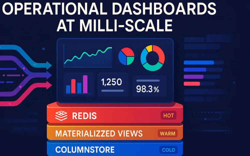
A more intentional approach—now common in high-throughput platforms—is the Triad Architecture. It uses three complementary layers, each built for a different “temperature” of data.

1.3.1 Columnstore (Cold Path)

Columnar analytical engines such as ClickHouse or Apache Pinot are optimized for heavy workloads:

• Scanning billions of rows
• Running window functions
• Performing large groupings
• Computing time-based metrics

These engines are extremely efficient because they store columns separately, compress data aggressively, and execute queries using vectorized processing. They handle historical analysis with predictable performance, even at terabyte scale.

1.3.2 Materialized Views (Warm Path)

Materialized Views act as a middle layer between real-time data and historical storage. They precompute expensive operations so that dashboard queries don’t have to.

Examples include:

• Hourly sales totals
• Delay averages by region
• One-minute buckets of events
• Joins between fact and dimension tables

This produces stable intermediate datasets that are fast to query and cheap to maintain.

1.3.3 Redis Read Models (Hot Path)

Redis serves the data that must be returned instantly. It stores not raw data, but the exact answers the dashboard needs:

• Counters
• Rolling windows
• Active states
• Prebuilt JSON for charts

Because Redis is in-memory and specializes in constant-time operations, it consistently delivers single-digit millisecond responses.

1.3.4 Triad Summary

Layer	Strength	Refresh Model	Use Cases
Redis (Hot)	Millisecond reads	Real-time updates	Live counters, recent activity
Materialized Views (Warm)	Pre-aggregated accuracy	Frequent incremental runs	Trends, KPIs, join-heavy metrics
Columnstore (Cold)	Heavy analytics	Batch ingestion	Long-term & historical analysis

By splitting work across these specialized layers, the system can stay fast at peak load, maintain accurate data, and keep costs under control. The triad allows teams to build dashboards that operate reliably at milli-scale—where every millisecond matters.

---

2 Architectural Blueprints: The Hot, Warm, and Cold Paths

The Triad Architecture works because not all data needs to be handled the same way. Some metrics must update instantly, others only need minute-level freshness, and historical data can be recalculated in batches. Treating everything as “real-time” creates bottlenecks. Instead, the system divides data into hot, warm, and cold paths based on freshness requirements and processing cost. These paths determine which engine stores the data, how it’s updated, and how dashboards read it.

This section explains what each path does, how events flow to the correct tier, and why clean separation between writing and reading is essential for predictable milli-scale performance.

2.1 Data Temperature Classification

The idea of “data temperature” gives teams a simple mental model: Hot = needed right now. Warm = needed soon but not instantly. Cold = needed for depth, not immediacy.

Each temperature zone matches a different workload and a different engine in the triad: Redis for hot, Materialized Views for warm, and Columnstores for cold.

2.1.1 Hot Path (Redis)

Hot-path data is what the dashboard must return without thinking—simple values that represent the most current state of the system. This includes:

• Current active users or devices
• Counters for the last few minutes
• Rolling “orders per minute” style metrics
• Top lists that refresh continuously

Redis is ideal here because it doesn’t calculate anything—it simply returns values already stored in memory. Its structures (Hashes, Sorted Sets, HyperLogLog) and atomic operations allow these numbers to update efficiently as events arrive.

A typical update from a Kafka consumer looks like this:

# Python pseudo-code
redis.hincrby("kpi:sales:region:us", "count", 1)
redis.hincrbyfloat("kpi:sales:region:us", "amount", order_total)

This keeps Redis aligned with incoming events, so dashboard widgets can fetch answers in 1–5 ms.

2.1.2 Warm Path (Materialized Views)

Warm-path data comes from raw events but doesn’t need to update immediately. These metrics usually require heavier processing—joins, buckets, groupings—but they can tolerate a small delay.

Typical examples include:

• Hour-over-hour sales
• Delay averages by region
• One-minute aggregated buckets
• Multi-table enrichments

Materialized Views work well here because they turn expensive operations into precomputed tables. The dashboard reads from already-shaped data rather than raw logs.

A ClickHouse Materialized View for one-minute order rollups might look like:

CREATE MATERIALIZED VIEW mv_orders_1m
ENGINE = AggregatingMergeTree()
PARTITION BY toDate(created_at)
ORDER BY (toStartOfMinute(created_at), region)
AS
SELECT
    toStartOfMinute(created_at) AS ts,
    region,
    sumState(amount) AS amount_state
FROM orders
GROUP BY ts, region;

These tables stay small, structured, and predictable—ideal for warm-path queries.

2.1.3 Cold Path (Columnstore / Data Lake)

Cold-path data refers to historical or analytical workloads that don’t need fast turnaround but do require deep coverage:

• Multi-year patterns
• SLA and compliance reporting
• Historical baseline comparisons
• Full-route or transaction histories

Columnstores shine here because they compress data efficiently and execute analytical queries with vectorized processing across distributed nodes.

A typical cold-path query might compute a city-level delay average across a year:

SELECT city, avg(delay_minutes)
FROM fleet_events
WHERE event_date >= today() - 365
GROUP BY city;

The cold path is where detail lives; the hot and warm layers expose summaries derived from it.

2.2 The Ingestion Router

In the triad, ingestion is intentionally split. A single event may feed all three paths: immediately to Redis, then to Materialized Views, and finally to the full historical dataset. This prevents the dashboard from overworking any single engine.

An Ingestion Router—usually implemented with Kafka, Debezium, or a similar streaming platform—controls this fan-out. It ensures each consumer group handles only the work relevant to its layer.

2.2.1 Dual-Path Example

Suppose a new order event arrives in Kafka:

{
  "order_id": 123,
  "region": "us",
  "amount": 49.95,
  "created_at": "2025-02-01T12:04:00Z"
}

Two consumers process this event:

• Hot-path consumer: Updates Redis counters instantly
• Cold/warm-path consumer: Inserts the event into ClickHouse, where Materialized Views will aggregate it

2.2.2 Pseudo-code for Split Processing

Both paths operate independently:

for event in kafka.consume("orders"):

    # --- Hot Path ---
    redis.hincrby("kpi:sales:region:"+event.region, "count", 1)
    redis.hincrbyfloat("kpi:sales:region:"+event.region, "amount", event.amount)

    # --- Cold/Warm Path ---
    clickhouse.insert("orders", event)

This division gives each path what it needs without forcing one to wait for the other.

2.2.3 Why Not Use a Single Consumer?

A single consumer doing everything is brittle. Dedicated consumers make the system healthier because they provide:

• Independent scaling — warm path might need more partitions than hot path
• Fault isolation — Redis updates can continue even if ClickHouse temporarily slows
• Predictable SLAs — each layer has its own timing requirements
• Simpler monitoring — lag per path becomes clear and diagnosable

When the pipeline grows, this separation prevents ingestion from dragging down dashboards.

2.3 State Management: Write vs. Read Side

A core principle of milli-scale dashboards is keeping writing and reading strictly separate. The write side handles ingestion and transformation. The read side answers questions without doing extra work. This mirrors CQRS, but applied at the data platform level instead of the application layer.

2.3.1 Write-Side Responsibilities

The write side does the heavy lifting:

• Consumes events
• Normalizes and enriches them
• Feeds Materialized Views
• Appends to columnstore tables
• Updates Redis read models

This ensures correctness and predictability before data ever reaches the dashboard.

2.3.2 Read-Side Behavior

The read side should be as lightweight as possible. For dashboards, this means:

• Redis lookups for hot data
• Simple SELECTs against warm views
• Optional joins with small dimension tables
• No heavy transformations

If a dashboard endpoint is still building results at runtime, the architecture is not yet aligned with milli-scale goals.

2.3.3 Example Read-Side SQL (Warm Path)

A typical warm-path query looks like this:

SELECT ts, region, sumMerge(amount_state) AS amount
FROM mv_orders_1m
WHERE ts >= now() - INTERVAL 1 HOUR
ORDER BY ts;

It completes quickly because:

• Aggregation was already done in the write path
• The query only merges stored states
• The range is bounded and well-indexed

This separation of concerns—write first, read fast—is what allows dashboards to remain stable and consistent under high load.

---

3 Columnstore & Materialized Views: The Heavy Lifters

Once a system reaches milli-scale expectations, even medium-sized aggregations become too expensive for a transactional database. This is where columnstores and Materialized Views carry most of the load. The cold path (columnstore) handles deep history and high-volume analytics, while the warm path (Materialized Views) ensures dashboards read from pre-shaped, efficient tables instead of raw event logs. This section explains how to choose the right engine, how pre-aggregation works in practice, and how layered views create stable, predictable interfaces for dashboard APIs.

3.1 Choosing the Right Engine: ClickHouse vs. Apache Pinot

Columnstores are popular for operational analytics because they only read the columns they need and compress data aggressively. They’re built for the kind of wide scans and repeated group-bys that dashboards rely on. Among open-source options, ClickHouse and Apache Pinot are the most commonly deployed.

3.1.1 ClickHouse

ClickHouse excels when the system ingests data in batches and needs strong analytical capabilities. It supports:

• High-throughput bulk inserts
• Vectorized execution for fast scans
• Materialized Views powered by AggregatingMergeTree
• Complex SQL including JOINs and window functions

Strengths:

• Mature optimizer
• Flexible schemas and table engines
• Built-in replication and sharding through Distributed tables
• Strong ecosystem for ETL and warm-path aggregation

Limitations:

• Real-time ingestion is possible but requires more tuning compared to a streaming-native engine

ClickHouse pairs naturally with Redis when the ingestion router (Section 2) delivers large volumes of raw events every second.

3.1.2 Apache Pinot

Pinot is designed for scenarios where events must be queryable almost immediately—often within seconds of being emitted. It emphasizes:

• Real-time ingestion directly from Kafka
• Ultra-low-latency OLAP queries
• The StarTree index for fast, pre-aggregated lookups
• Streaming-friendly architecture

Strengths:

• Built for real-time dashboards
• Efficient rollups
• Minimal ingestion lag

Limitations:

• SQL surface is narrower than ClickHouse
• Operationally more complex (controller/broker/server components)

Pinot is typically chosen for “live analytics” products—behavior tracking, monitoring platforms, IoT streams—where freshness is more important than complex SQL.

3.1.3 Decision Criteria

To decide which engine fits your dashboard, compare ingestion patterns and analytic needs:

Requirement	Best Choice
Very large batch inserts (≥1M rows/sec)	ClickHouse
Real-time ingestion from Kafka with minimal delay	Pinot
Complex SQL joins or calculations	ClickHouse
StarTree-based low-latency rollups	Pinot
Strong Materialized View ecosystem	ClickHouse

Most milli-scale dashboards end up with either ClickHouse + Redis or Pinot + Redis, depending on whether ingestion is batch-oriented or stream-oriented.

3.2 AggregatingMergeTree & IVM: Precomputing Heavy Queries

To keep warm-path queries in the 10–50 ms range, expensive aggregations must be computed in the write path instead of the read path. Pre-aggregation turns what used to be million-row scans into lightweight merges.

Two widely used approaches are ClickHouse’s AggregatingMergeTree and PostgreSQL’s Incremental View Maintenance (IVM).

3.2.1 ClickHouse AggregatingMergeTree

AggregatingMergeTree stores aggregation states instead of fully computed numbers. These states compress well and merge quickly, making them ideal for rollups like “orders per region per minute” or “average delay by hour.”

Schema Example (matching the earlier order flow):

CREATE TABLE orders_agg
(
    ts DateTime,
    region String,
    amount_state AggregateFunction(sum, Float64),
    count_state AggregateFunction(count, UInt64)
)
ENGINE = AggregatingMergeTree()
PARTITION BY toDate(ts)
ORDER BY (ts, region);

Materialized View populating it:

CREATE MATERIALIZED VIEW mv_orders_agg
TO orders_agg
AS
SELECT
    toStartOfMinute(created_at) AS ts,
    region,
    sumState(amount) AS amount_state,
    countState() AS count_state
FROM orders
GROUP BY ts, region;

Querying pre-aggregated data:

SELECT
    ts,
    region,
    sumMerge(amount_state) AS total_amount,
    countMerge(count_state) AS total_orders
FROM orders_agg
WHERE ts >= now() - INTERVAL 1 HOUR
GROUP BY ts, region
ORDER BY ts;

ClickHouse now performs a simple “merge of states” instead of recomputing sums across raw logs. This is why warm-path queries maintain predictable latency even as the dataset grows by billions of rows.

3.2.2 PostgreSQL Incremental View Maintenance (IVM)

For teams that already rely heavily on PostgreSQL, IVM offers a warm-path alternative without introducing a new engine. It updates Materialized Views incrementally as new events arrive, avoiding full refreshes.

Example:

CREATE MATERIALIZED VIEW mv_hourly_sales
WITH (incremental = true) AS
SELECT
    date_trunc('hour', created_at) AS hour,
    region,
    SUM(amount) AS total_amount
FROM orders
GROUP BY 1,2;

IVM works best for moderate volumes where PostgreSQL remains the system of record. It does not match ClickHouse’s throughput, but it’s a practical option when introducing a columnstore is not yet necessary.

3.2.3 When to Use Which

Scenario	Recommended Engine
Heavy ingestion with billions of rows/day	ClickHouse
Mid-size OLTP-backed analytics	PostgreSQL IVM
Real-time Kafka streams	Pinot

This keeps warm-path design consistent with the ingestion profiles introduced in Section 2.

3.3 View Layering Strategy

A common mistake is to build a single “all-purpose” aggregated table and have the dashboard query it directly. That pattern doesn’t scale. Instead, a layered view model ensures each stage of transformation produces a stable, predictable shape that downstream layers can depend on.

3.3.1 Layer 1: Raw Data

The raw layer stores immutable events exactly as they arrive from the ingestion router.

CREATE TABLE orders_raw
(
    order_id UInt64,
    region String,
    amount Float64,
    created_at DateTime
)
ENGINE = MergeTree()
PARTITION BY toDate(created_at)
ORDER BY (created_at, order_id);

This table grows quickly but is optimized for fast inserts and history retention.

3.3.2 Layer 2: Derived Views

The derived layer holds pre-aggregated metrics, usually computed via Materialized Views. These match the warm-path use cases described earlier—1-minute buckets, 5-minute windows, regional rollups.

CREATE MATERIALIZED VIEW mv_orders_1m
TO orders_1m
AS
SELECT
    toStartOfMinute(created_at) AS ts,
    region,
    sumState(amount) AS amount_state
FROM orders_raw
GROUP BY ts, region;

These tables are small, indexed well, and stable—exactly what milli-scale dashboards need.

3.3.3 Layer 3: Presentation Views

The last layer shapes the data into the exact format expected by the dashboard API. This avoids per-request transformations and ensures the query surface remains stable even if upstream schemas evolve.

CREATE VIEW v_orders_dashboard AS
SELECT
    ts,
    region,
    sumMerge(amount_state) AS revenue,
    revenue 
       / NULLIF(lagInFrame(revenue) OVER(PARTITION BY region ORDER BY ts), 0)
       AS hour_over_hour_growth
FROM orders_1m
ORDER BY ts;

This view presents clean, ready-to-serve KPIs—no additional calculations needed at query time.

Presentation views complete the workflow described in Sections 1 and 2: Raw events → Derived rollups → Dashboard-ready answers.

---

4 Redis Read Models: Engineering for Sub-Millisecond Access

Redis sits at the top of the triad because it solves the problem nothing else can: answering operational questions in a few milliseconds, even when the system is under pressure. To achieve that, Redis cannot behave like a traditional database. It doesn’t run joins, scans, or aggregations. It simply returns values that were already computed by the write side.

This section explains how to model Redis keys around dashboard questions, how probabilistic structures keep memory usage low, and how Lua scripting provides safe updates under concurrency. Together, these patterns make Redis a reliable hot path for milli-scale dashboards.

4.1 The “Answer-First” Schema Design

A Redis read model begins with the question the dashboard needs to answer—not with tables, entities, or relationships. The write side prepares the answer in advance, and Redis stores it under a predictable key. The dashboard then retrieves that key directly with no transformation.

For example, if the system needs the total sales for the US region over the last hour, the key might be:

dashboard:kpi:sales:region:us:1h

The value stored under this key is the computed number, not the underlying events. When the dashboard queries it, Redis returns the value immediately:

result = redis.get("dashboard:kpi:sales:region:us:1h")
return {"kpi": float(result)}

This is the same pattern used in earlier sections: the write side (via Kafka consumers) updates Redis as events come in, and the read side performs only a simple lookup.

Complex widgets use the same approach. Consider a chart showing per-minute sales for the last hour. Instead of computing buckets at query time, the write side stores a ready-to-use structure:

dashboard:chart:sales:region:us:1h

A simple C# increment during ingestion might look like:

var db = redis.GetDatabase();
string key = $"dashboard:kpi:sales:region:{region}:total";
await db.StringIncrementAsync(key, amount);

By following this pattern, the hot path stays predictable: Redis always returns exactly what the dashboard needs, with no extra processing.

4.2 Probabilistic Data Structures

Some real-time metrics involve high-cardinality sets—unique drivers, unique visitors, device IDs, etc. Storing every element in a Redis Set can consume memory quickly. Probabilistic structures help maintain accuracy while keeping memory usage manageable. They are ideal for operational dashboards where the exact value isn’t required for every second-by-second view.

4.2.1 HyperLogLog for Unique Counts

HyperLogLog (HLL) estimates the number of unique items in a set while storing only a few kilobytes of state. This allows the system to track things like unique drivers reporting in the last hour without creating massive sets.

redis.pfadd("fleet:unique:drivers:1h", driver_id)

Fetching the estimate is just as simple:

unique_drivers = redis.pfcount("fleet:unique:drivers:1h")

For operational dashboards—where trends matter more than perfect precision—this trade-off is both practical and cost-efficient.

4.2.2 Bloom Filters for Membership Checks

Bloom filters allow quick “might exist” checks with no false negatives and a small number of false positives. They reduce the need to query Columnstores or lookup tables for every identity check.

Common uses include:

• Checking if a vehicle ID is active
• Validating whether a customer ID exists
• Preventing unnecessary cold-path lookups

Example using RedisBloom:

redis.bf().create("active:vehicles", 0.01, 100000)
redis.bf().add("active:vehicles", vehicle_id)

if redis.bf().exists("active:vehicles", vehicle_id):
    return "active"

This pattern avoids unnecessary reads from the warm or cold path and helps keep latency predictable.

4.2.3 Combining HLL With Warm-Path Data

HLL gives fast estimates, but the warm path often maintains precise aggregates. Many systems combine both:

• Use HLL for real-time counters
• Periodically overwrite Redis with exact numbers from Materialized Views

This matches the “self-healing” strategy introduced in Section 5, keeping Redis fast and correct.

4.3 Lua Scripting for Atomicity

When multiple ingestion consumers update Redis at the same time, race conditions can appear—especially for rolling counters or metrics that depend on ordering. Lua scripts solve this by running atomically inside Redis, guaranteeing the update logic completes safely as a single operation.

A simple example: updating a rolling KPI while preventing negative values when events arrive out of order.

-- update_kpi.lua
local key = KEYS[1]
local delta = tonumber(ARGV[1])
local current = tonumber(redis.call("GET", key)) or 0
local new = current + delta
if new < 0 then new = 0 end
redis.call("SET", key, new)
return new

Called from Python:

script = redis.register_script(open("update_kpi.lua").read())
new_value = script(keys=["dashboard:kpi:sales:region:us:1h"], args=[-5])

Lua is also useful for multi-step updates where atomicity matters—such as incrementing a counter and updating a timestamp together:

-- atomic_multi_update.lua
local countKey = KEYS[1]
local tsKey = KEYS[2]
local increment = tonumber(ARGV[1])
redis.call("INCRBYFLOAT", countKey, increment)
redis.call("SET", tsKey, ARGV[2])
return {redis.call("GET", countKey), redis.call("GET", tsKey)}

By centralizing logic inside Redis, the hot path avoids race conditions and keeps metrics consistent even during heavy ingestion.

4.4 Redis Stack & JSON

Many dashboard widgets need structured output—labels, values, drill-down metadata—not just single numbers. RedisJSON stores full widget payloads so the frontend can fetch a complete object in one request.

Example payload for a revenue chart:

{
  "labels": ["10:00", "10:01", "10:02"],
  "values": [1200.5, 1300.0, 1150.25],
  "region": "us"
}

Writing it to Redis:

redis.json().set("dashboard:chart:revenue:us:1h", "$", payload)

Fetching a portion of the JSON:

result = redis.json().get("dashboard:chart:revenue:us:1h", "$.values")

C# example:

var db = redis.GetDatabase();
await db.JsonSetAsync("dashboard:chart:revenue:us:1h", "$", payload);
var values = await db.JsonGetAsync("dashboard:chart:revenue:us:1h", "$.values");

This approach keeps the read path minimal. The write path prepares a fully rendered widget payload, and the dashboard retrieves it in a single call—no reshaping, joining, or filtering required.

---

5 Refresh Strategies & Consistency Windows

Redis gives us speed, but it doesn’t create truth—it only reflects what the write side tells it. The warm and cold paths still hold the authoritative results, and Redis must be kept in sync with them. To do that without hurting performance, the system relies on refresh strategies and consistency windows—clear rules that define how fresh each metric needs to be.

This section explains how to set those expectations, how real-time and batch updates work together, and when to use eager or lazy loading to keep Redis both accurate and efficient.

5.1 The “Near-Real-Time” Contract

Operational dashboards don’t need perfect real-time precision; they need predictable freshness. Users should always know how current the data is, even if it’s not accurate to the millisecond.

A typical contract might look like:

• Live counters update every second
• Rolling one-minute aggregates lag by up to one minute
• Hourly summaries refresh every five minutes

For example, a logistics operator understands that the “Vehicles on Route” widget updates almost instantly, while “Average Delay by City” is based on aggregated data that might be a couple of minutes behind.

The system enforces this contract by assigning refresh intervals to each view. A one-minute view may run every 30 seconds; a 24-hour summary may run every 10 minutes. The dashboard API doesn’t worry about freshness or recalculating data—it simply retrieves whatever the refresh cycle has prepared.

A simple scheduled refresh might look like this:

def refresh_1min_aggregation():
    result = client.execute("SELECT * FROM v_orders_1m_last_hour")
    payload = format_for_redis(result)
    redis.json().set("dashboard:chart:orders:1m", "$", payload)

These processes run independently from dashboard reads. The API never regenerates values; it only returns the latest prepared answer stored in Redis.

5.2 Lambda vs. Kappa Architecture Refined

The triad model borrows from both Lambda and Kappa architectures but adapts them to focus on low-latency dashboards. The key refinement is simple: Redis stores two kinds of values.

• Real-time, unconfirmed values: updated by the ingestion router in the hot path
• Confirmed values: periodically overwritten by warm or cold path aggregations

This dual-write pattern lets Redis stay fresh in the moment while still correcting drift over time.

5.2.1 Speed Layer

The speed layer updates Redis immediately from event streams. These updates represent the most recent activity—seconds or even milliseconds old. They prioritize responsiveness over complete accuracy.

Example:

redis.hincrby("metrics:orders:1m", "count", 1)

This value is fresh but can drift slightly because:

• Some events arrive late
• Duplicates may temporarily inflate counts
• Ordering isn’t guaranteed in the stream

That’s acceptable, because the batch layer will fix these discrepancies.

5.2.2 Batch Layer (Self-Healing)

The batch layer periodically overwrites Redis keys with authoritative numbers from ClickHouse or Pinot. This corrects drift from the speed layer and ensures long-term accuracy.

rollups = client.execute("SELECT * FROM v_orders_1m")

for row in rollups:
    key = f"metrics:orders:region:{row.region}:1m"
    redis.set(key, row.total_amount)

During the window between two batch updates, Redis is “near-real-time.” Once the batch overwrite occurs, it becomes exact again. This is the self-healing pattern: real-time updates keep dashboards responsive, and batch updates keep them accurate.

5.2.3 Unified Event Stream (Kappa Refinement)

Many modern systems follow a Kappa-like approach where both the speed layer and the batch layer consume from the same event stream. The difference lies in processing strategy:

• The speed layer acts immediately
• The batch layer groups or aggregates events into windows

This avoids maintaining two separate pipelines while still enabling dual-refresh behavior.

5.3 Lazy vs. Eager Loading

Redis is fast, but its memory isn’t unlimited. Some dashboard widgets should be precomputed, while others should only be built when users request them. The challenge is finding the balance between performance and resource usage.

5.3.1 Eager Loading

Eager loading pre-populates Redis with complete payloads right after Materialized Views or ETL processes finish. This makes dashboard responses instantaneous, even during heavy traffic.

payload = build_dashboard_payload()
redis.json().set("dashboard:orders:summary", "$", payload)

Eager loading is ideal when:

• A widget is frequently viewed
• The computation is expensive to recreate
• Tight consistency windows are required

It ensures that the dashboard never triggers expensive operations during peak load.

5.3.2 Lazy Loading with Cache Stampede Protection

Lazy loading computes the value only when a user first requests it. This saves memory and processing time for less frequently accessed widgets. But without safeguards, multiple users could trigger the same expensive computation simultaneously.

A simple locking mechanism avoids this:

if redis.setnx("lock:dashboard:orders:summary", "1"):
    redis.expire("lock:dashboard:orders:summary", 30)
    payload = compute_summary()
    redis.json().set("dashboard:orders:summary", "$", payload)
    redis.delete("lock:dashboard:orders:summary")
else:
    # Another worker is generating the value
    time.sleep(0.1)

This pattern prevents “cache stampedes,” keeps Redis memory usage controlled, and adapts well to dashboards with varied usage patterns.

Lazy loading also works well with TTL-based keys. When a key expires naturally, the next request triggers a controlled refresh rather than a burst of concurrent updates.

---

6 Resilience: Back-Pressure and Flow Control

A dashboard architecture that performs well only when traffic is stable isn’t production-ready. Real systems deal with unpredictable spikes: a sudden GPS burst from thousands of trucks, a marketing event that triples web traffic, or a bulk import from an external partner. If ingestion isn’t controlled, warm-path processes can overload, Redis refreshes fall behind, and the cold path starts accumulating lag.

Resilience comes from treating the system as a set of coordinated flows rather than a monolithic pipe. The goal isn’t to eliminate spikes—those are inevitable—but to make sure they don’t ripple through the entire stack or degrade the user experience.

6.1 Handling Ingestion Spikes

During spikes, the warm path is usually the first layer to feel pressure. Materialized Views perform merges, bucket computations, and sometimes joins. These operations are efficient but still heavier than simple inserts to ClickHouse or direct increments to Redis. When ingestion volume rises sharply, repeatedly refreshing warm-path views can slow everything down.

A practical way to prevent this is a circuit breaker inside the ingestion consumer. Instead of continuing to trigger warm-path logic when the system is strained, the breaker temporarily pauses refreshes based on:

• Kafka consumer lag
• ClickHouse insert latency
• CPU or I/O thresholds

Cold-path inserts continue uninterrupted, and Redis hot-path updates remain instant. Only the warm-path refresh step is paused until the system recovers.

Example Python circuit-breaker logic:

MAX_LAG = 50000
MAX_LATENCY_MS = 200

def should_break(lag, latency):
    return lag > MAX_LAG or latency > MAX_LATENCY_MS

for batch in kafka.consume_batches("gps-stream"):
    lag = kafka.get_consumer_lag()
    latency = measure_clickhouse_latency()

    if should_break(lag, latency):
        logger.warning("Breaker open: skipping MV refresh")
        clickhouse.insert("gps_raw", batch)
        continue

    clickhouse.insert("gps_raw", batch)
    trigger_mv_refresh_if_needed()

In this pattern:

• Redis continues receiving live updates
• ClickHouse continues storing raw events
• Materialized Views skip refreshes until the system stabilizes

Warm-path metrics may lag slightly, but the dashboard remains responsive—exactly what milli-scale reliability requires.

A lightweight C# version:

if (lag > maxLag || latency > maxLatency)
{
    breaker.Open();
}
else
{
    breaker.Close();
}

if (!breaker.IsOpen)
{
    TriggerMaterializedViewRefresh();
}

Circuit breakers prevent cascading failures and make the ingestion pipeline self-stabilizing.

6.2 Shedding Load

Sometimes ingestion spikes exceed what the system can reasonably handle in real time. Instead of letting the entire pipeline fail, the system intentionally reduces work—a technique known as load shedding.

For many operational metrics, perfect precision isn’t necessary in the hot path. Examples include:

• Vehicle telemetry frequency
• Session counts
• Orders-per-minute spikes
• Sensor readings from dense IoT deployments

Sampling is the simplest shedding strategy. For example, during extreme load the system might process only 10% of incoming telemetry for real-time counters:

if random.random() > 0.1:
    continue  # skip this event under pressure

Key points:

• Redis still reflects trends accurately
• ClickHouse still receives all raw events for cold-path correctness
• Warm-path refreshes run at a stable pace

Sampling helps ensure Redis doesn’t fill up with unnecessary updates and warm-path merges don’t fall behind.

Another common technique is pausing or slowing warm-path refreshes when CPU or storage pressure increases. Since Redis holds near-real-time approximations, dashboards continue working smoothly even if warm-path queries are temporarily delayed.

This is the same principle used earlier: the warm path is important, but it should never dictate system health on its own.

6.3 Dead Letter Queues (DLQ)

Even well-designed pipelines encounter malformed messages, unexpected schemas, or events that simply can’t be processed. Stopping the pipeline for a handful of bad events isn’t an option at milli-scale. A Dead Letter Queue (DLQ) ensures the system can keep moving while still capturing problematic events for later review.

A DLQ typically includes:

• A dedicated Kafka topic like dlq.gps or dlq.orders
• Metadata describing the failure
• A replay mechanism for reprocessing events after fixes

Example in Python:

try:
    transformed = transform_event(event)
    clickhouse.insert("gps_raw", transformed)
except Exception as ex:
    dlq_event = {"event": event, "error": str(ex)}
    kafka.produce("dlq.gps", dlq_event)

This approach keeps ingestion flowing:

• Redis continues receiving hot-path updates
• ClickHouse persists the majority of raw events
• Warm-path calculations skip only the bad entries

DLQ data is also a valuable diagnostic tool. It shows exactly which devices, integration points, or event formats are causing issues. Operators can replay DLQ entries once schema corrections or transformation fixes are deployed.

For warm-path failures—such as aggregation errors—the system often proceeds without blocking, ensuring throughput remains unaffected. The cold path still captures full fidelity, and the self-healing pattern described in Section 5 ensures Redis eventually receives corrected values.

---

7 Real-Life Implementation: “Live Logistics Fleet Dashboard”

To make the triad architecture concrete, consider a real-world logistics dashboard that tracks a fleet of roughly 50,000 trucks. Each vehicle streams GPS data every few seconds. Dispatch teams rely on this dashboard to monitor active trucks, spot delays, and react to exceptions as they happen. The workload mixes high-volume ingestion with strict latency and accuracy expectations, making it an ideal example of a system that must operate at milli-scale.

7.1 The Use Case

Each truck publishes:

• Current GPS coordinates
• Route status (departed, arrived, delayed)
• ETA or delay changes
• Geofence transitions

A single region can generate tens of thousands of messages per minute. Dispatchers need to see:

• Which trucks are currently active
• Delay averages by city
• Vehicles entering or leaving their zones
• A live event feed showing recent departures, arrivals, and exceptions

These are exactly the kinds of metrics that benefit from the triad model: Redis handles live snapshots and counters, Materialized Views provide stable aggregates, and ClickHouse stores the full event history.

7.2 The Stack

The architecture mirrors what we’ve described in earlier sections, applied to fleet data.

Ingest: Apache Kafka

Every GPS update and route event enters Kafka first. Vehicle IDs act as partition keys so updates for the same truck stay ordered. Planning systems (like deliveries or updated ETAs) push changes through CDC connectors, which also land in Kafka topics.

This gives the ingestion router a unified event stream, making it easier to direct each update to the hot, warm, or cold path.

Store: ClickHouse With Materialized Views

All raw GPS events land in a ClickHouse table. Materialized Views then prepare warm-path rollups:

• One-minute route aggregates
• Average delay by city
• City-level or region-level delay distributions

Because the warm path precomputes these metrics, dashboard queries against ClickHouse remain predictable—no large joins or wide scans.

Cache: Redis Streams and Hashes

Redis handles the operational views:

• Redis Hashes store the latest state for each truck
• Redis Streams store recent activity events for the dashboard’s live feed

This gives the frontend instant access to both a “snapshot” view and a “recent events” feed without touching the warm or cold path.

7.3 The Code Snippet Logic

A single Kafka consumer can update all three layers consistently. Following the same pattern used in previous sections, it updates Redis first (hot path) and then writes the raw event to ClickHouse (cold path). The warm path updates automatically through Materialized Views.

Python Example: Write-Through Logic

for event in kafka.consume("gps-updates"):

    truck_id = event["truck_id"]
    location = event["location"]
    delay = event["delay_minutes"]

    # --- Hot Path ---
    # Update the truck’s latest known state
    redis.hset(f"truck:{truck_id}:state", mapping={
        "lat": location["lat"],
        "lon": location["lon"],
        "delay": delay,
        "updated_at": event["timestamp"]
    })

    # Track unique active trucks in the last hour
    redis.pfadd("fleet:active:trucks:1h", truck_id)

    # Add this event to the scrolling live feed
    redis.xadd("fleet:feed", {
        "truck_id": truck_id,
        "delay": delay,
        "ts": event["timestamp"]
    })

    # --- Cold/Warm Path ---
    # Insert the raw event into ClickHouse
    clickhouse.insert("gps_raw", event)

This matches the patterns from earlier sections:

• Redis receives the immediate operational values
• ClickHouse receives the authoritative raw record
• Materialized Views generate aggregated metrics automatically

C# Example: Structured Update

var db = redis.GetDatabase();

foreach (var evt in kafka.Consume("gps-updates"))
{
    string truckKey = $"truck:{evt.TruckId}:state";

    // Hot path: update the truck’s current snapshot
    db.HashSet(truckKey, new HashEntry[]
    {
        new HashEntry("lat", evt.Lat),
        new HashEntry("lon", evt.Lon),
        new HashEntry("delay", evt.Delay),
        new HashEntry("updated_at", evt.Timestamp)
    });

    // Track unique active vehicles
    db.Execute("PFADD", "fleet:active:trucks:1h", evt.TruckId);

    // Add event to live event stream
    db.StreamAdd("fleet:feed", new NameValueEntry[]
    {
        new NameValueEntry("truck_id", evt.TruckId),
        new NameValueEntry("delay", evt.Delay),
        new NameValueEntry("ts", evt.Timestamp)
    });

    // Cold path insert
    clickHouseClient.Insert("gps_raw", evt);
}

Once these values are in Redis and ClickHouse:

• The dashboard retrieves the truck snapshot from the Redis Hash
• It reads recent events from the Redis Stream
• It queries Materialized Views for delay trends or city rollups

This structure keeps the dashboard fast even when ingestion spikes. The hot path remains lightweight and instantaneous, the warm path produces clean aggregates, and the cold path maintains the full history needed for analytics and compliance.

---

8 Conclusion & Future Outlook

As operational dashboards become central to real-time decision-making, expectations for performance rise accordingly. Dispatchers, analysts, and operations teams now rely on dashboards as their primary interface into live systems. For these workloads, “fast most of the time” is not enough. The architecture must deliver predictable, millisecond-level responsiveness even when ingestion surges or data volumes grow sharply.

The triad architecture—Redis for hot-path answers, Materialized Views for warm-path aggregations, and Columnstores for cold-path analytics—continues to be the most reliable pattern in high-volume environments such as logistics, fintech, retail, and IoT telemetry. No single engine can serve all these workloads efficiently. Each tier plays a distinct role, and together they create a stable and scalable foundation for operational dashboards.

8.1 The Consolidation Trend

A new class of systems—such as Materialize and Rockset—has begun merging stream processing, Materialized Views, and analytical querying into a single engine. These platforms offer:

• Incremental view updates
• SQL-first development
• Real-time ingestion
• Low-latency lookups over changing data

For organizations that don’t need sub-millisecond access or cannot maintain multiple specialized systems, these tools reduce architectural complexity. They effectively blend the warm and cold paths into one engine.

However, even with these advancements, Redis still remains unmatched for ultra-low-latency operational reads. When dashboards require instantaneous snapshots—like truck locations, live counters, or rolling one-minute KPIs—Redis continues to outperform consolidated solutions by a wide margin.

This is why the triad model remains relevant: it allows teams to combine the strengths of specialized systems rather than rely on a single tool to do everything. In large-scale, high-frequency environments—like the 50,000-truck fleet example used throughout this article—this separation of concerns remains essential.

8.2 Checklist for Architects

When assessing or designing an operational dashboard, architects can use the following checklist to verify that the system is aligned with milli-scale expectations:

1. Are any dashboard widgets querying OLTP tables directly? If so, address this immediately. Transactional databases cannot provide consistent, low-latency reads under dashboard load.

2. Does every KPI or widget map to a specific Redis key or read model? If not, the hot path isn’t answer-first. Redis should store the answer—not the raw data required to compute it.

3. Are Materialized Views shaped specifically for dashboard queries? If warm-path SQL still involves joins, filters over large ranges, or heavy group-bys, the system will become unpredictable under load.

4. Can the ingestion pipeline absorb sudden spikes? Look for circuit breakers, sampling strategies, and DLQs. Without these, a short ingestion burst can snowball and degrade dashboard responsiveness.

5. Does Redis receive periodic, authoritative overwrites from ClickHouse or other cold/warm layers? Real-time increments drift over time. Without self-healing refresh cycles, Redis values eventually become inaccurate.

Teams that consistently follow these patterns build dashboards that stay fast and reliable even when event volume triples or user activity jumps unexpectedly. As expectations for real-time insight continue to grow, these architectural principles move from “nice to have” to essential.

The triad architecture provides a clear path forward: let each system do what it does best, maintain clean separation between hot, warm, and cold paths, and design read models that answer operational questions directly. This combination is what enables true milli-scale dashboards—systems that stay responsive when they matter most.