Graph Problems on Relational Systems: SQL Server Graph vs. Neo4j—When to Choose What

1 Introduction: The Inevitable Rise of Connected Data

Relational databases have been the backbone of enterprise systems for decades. They excel at structured, transactional workloads—think inventory management, financial ledgers, or HR systems. But as our world has become increasingly digital and interconnected, new classes of problems have emerged that are inherently relational in a different sense: they revolve around the connections between things. These are not just “foreign key joins”; they are deeply networked patterns—social graphs, fraud detection, logistics networks, recommendation engines, and knowledge graphs.

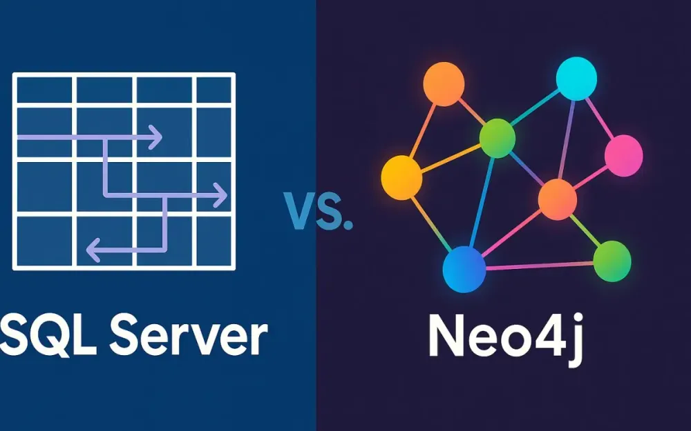
This shift from tabular to networked thinking explains why graph databases have moved from niche to mainstream. Yet for organizations entrenched in SQL Server or other relational systems, the big question is: Do we push our relational database to handle graph workloads, or do we adopt a specialized graph database like Neo4j?

This article begins by framing the problem, introduces the key players (SQL Server Graph vs. Neo4j), and then builds the mental models you need to evaluate which approach fits your architecture.

1.1 Beyond Rows and Columns

At its core, a relational system models data as rows in tables. Relationships are represented via foreign keys, and queries traverse these relationships through joins. This model works well when relationships are few and predictable: an Order belongs to a Customer; a LineItem belongs to an Order.

But modern data problems are often connection-heavy. Consider a fraud detection system. You don’t just want to know which credit card belongs to which customer. You want to explore:

• Which devices have been used across multiple accounts?
• Which IP addresses are shared by multiple customers?
• What is the shortest path between two accounts?
• Are there dense clusters of transactions suggesting a fraud ring?

In a relational schema, answering these questions often means joining dozens of tables, sometimes recursively. Performance suffers, queries become unwieldy, and reasoning about the data becomes a mental tax.

By contrast, graph models put relationships first. Each connection is a first-class citizen, stored and traversed efficiently. Instead of multi-join SQL queries, graph queries expressively declare patterns: “Find all customers within 3 hops of a known fraudster.” That’s the difference between trying to simulate relationships and making them the foundation of your data model.

1.2 The Core Problem

Let’s suppose you are leading a team that already runs mission-critical systems on SQL Server. Your developers are fluent in T-SQL, your operations team has battle-tested backups and HA strategies, and your business intelligence runs on SSRS or Power BI with SQL backends. Now, a new initiative emerges: building a recommendation engine, or monitoring supply-chain risks, or mapping a financial network for anti-money laundering compliance.

These problems share one property: they are graph-like. They require you to ask not just about data points, but about connections and paths. At this point, you have two choices:

1. Extend SQL Server with its Graph features. Pros: minimal disruption, no new infrastructure, same language and tooling. Cons: you’re using a system optimized for tables, not for graphs. Deep traversals will strain performance.

2. Adopt a native graph database like Neo4j. Pros: purpose-built for traversals, graph algorithms, and pattern matching. Rich ecosystem. Cons: operational overhead, new language (Cypher), new security and governance concerns, data integration challenges.

There’s no universal answer; the right choice depends on workload patterns, performance needs, team skills, and architectural goals. This article helps you reason about these trade-offs.

1.3 Meet the Contenders

SQL Server Graph

Microsoft introduced graph features in SQL Server 2017, extended in later versions including SQL Server 2022 and Azure SQL Database. The idea was pragmatic: let developers use familiar SQL tables, but with lightweight extensions to support graph-like semantics. Specifically:

• Node tables (AS NODE) to represent entities.
• Edge tables (AS EDGE) to represent relationships.
• The MATCH clause to express graph patterns.
• The SHORTEST_PATH function for traversals.

This approach is evolutionary, not revolutionary. It allows organizations to add graph querying capabilities without leaving the relational world. For workloads where graph analysis is a secondary concern, SQL Server Graph is often “good enough.”

Neo4j

Neo4j is the flagship native graph database. Unlike SQL Server Graph, it was built from the ground up around the property graph model. Its architecture enables index-free adjacency, where nodes directly reference their neighbors. Traversals are therefore O(depth) rather than O(depth × joins), making it performant on deeply connected data.

Neo4j’s Cypher query language is expressive and visual: (a)-[:FRIENDS_WITH*1..3]->(b) immediately conveys meaning. Beyond queries, Neo4j ships with a Graph Data Science (GDS) library, offering production-ready algorithms like PageRank, community detection, or graph embeddings for ML pipelines.

But adopting Neo4j means introducing a new technology stack. Teams must learn Cypher, rethink operational patterns, and often maintain synchronization between SQL and Neo4j systems. It’s a specialist tool—immensely powerful, but not always lightweight.

1.4 Article Goal & Target Audience

This article is written for senior developers, tech leads, and solution architects tasked with making technology choices that balance short-term pragmatism with long-term scalability.

Our goals are:

• To build clear mental models of graph data and problems.
• To explain, with concrete examples, how SQL Server Graph and Neo4j differ in design, querying, and performance.
• To surface trade-offs and decision criteria you can use in real-world architecture discussions.
• To walk through a practical scenario—a recommendation engine—and see how each system handles it.
• To end with a decision framework and best practices, including hybrid architectures.

By the end, you will not only understand when to choose what but also how to future-proof your graph strategy.

---

2 Foundational Concepts: Thinking in Graphs

Before we compare technologies, we need to ground ourselves in the property graph model—the dominant abstraction used by both SQL Server Graph and Neo4j. This model makes graphs practical for developers, allowing us to treat entities and relationships with equal importance.

2.1 The Property Graph Model

The property graph model has three main components: nodes, relationships (edges), and properties.

2.1.1 Nodes: The Entities

Nodes are the “things” in your domain. They can represent:

• A Customer in a retail system.
• A Device in a cybersecurity monitoring setup.
• A Protein in a biomedical research graph.

Each node can have labels, which act like types or categories. For example:

• (c:Customer {id: 123, name: 'Alice'})
• (p:Product {id: 456, category: 'Electronics'})

In SQL Server Graph, nodes are stored in node tables; in Neo4j, they are stored natively with labels.

2.1.2 Relationships: The Connections

Relationships (also called edges) represent how entities are linked. They are:

• Directed (in most systems): (Alice)-[:FRIENDS_WITH]->(Bob)
• Typed: The relationship has a semantic meaning like PURCHASED, LOCATED_IN, FOLLOWS.

In property graphs, relationships are first-class citizens. This contrasts with relational databases, where relationships are usually implied by foreign keys.

Example in Cypher:

(c:Customer {name: 'Alice'})-[:PURCHASED {date: '2025-09-05'}]->(p:Product {name: 'Laptop'})

In SQL Server Graph, relationships are stored in edge tables, which internally keep track of $from_id and $to_id.

2.1.3 Properties: The Context

Both nodes and relationships can carry properties as key-value pairs. This flexibility is critical:

• On a Customer node: {name: 'Alice', joined: '2021-03-15', loyaltyLevel: 'Gold'}
• On a PURCHASED relationship: {amount: 1299.99, channel: 'online'}

This allows storing not just what is connected, but how and why. For example, two users might both follow a celebrity, but one might have followed them yesterday (fresh connection) while another has been connected for years. That metadata is often essential.

2.1.4 Visual Thinking

One of the biggest shifts when adopting graphs is that you think in patterns. Queries resemble diagrams. For example, to find friends-of-friends, you’d literally draw (a)-[:FRIENDS_WITH]->(b)-[:FRIENDS_WITH]->(c). This is intuitive for developers and business stakeholders alike.

2.2 Common Graph Problems We Aim to Solve

Understanding the core types of graph problems clarifies why and when graphs are the right tool.

2.2.1 Pathfinding

Pathfinding asks: What is the shortest or optimal route between two nodes? Examples:

• Logistics: Find the shortest shipping route from factory to customer.
• Social networks: Determine if two users are connected within 4 degrees of separation.
• IT operations: Trace dependencies to find which downstream services will fail if a given API goes offline.

Relational queries can simulate pathfinding with recursive CTEs, but performance drops sharply as path length increases.

2.2.2 Centrality Analysis

Centrality measures influence or importance in a network. For example:

• Who are the most influential users in a social network? (High betweenness centrality.)
• Which airports are critical hubs in an airline network? (High degree centrality.)
• Which proteins act as bottlenecks in biological pathways?

Such algorithms require analyzing the entire structure of the graph, not just local neighborhoods. Native graph databases like Neo4j provide these algorithms off-the-shelf; relational systems generally require custom SQL implementations.

2.2.3 Community Detection

Community detection groups nodes into clusters of tight interconnections. This is useful for:

• Marketing: Segmenting customers not by demographics, but by actual behavioral connections.
• Fraud detection: Identifying rings of accounts working together.
• Research: Discovering collaboration clusters in scientific literature.

This is an area where the relational model struggles most, because you’re effectively asking about emergent structures not explicit in schema.

2.2.4 Pattern Matching & Recommendations

Graphs shine at discovering complex patterns:

• “Find customers who bought product A, whose friends also bought product A, and recommend product B that those friends purchased but the original customer hasn’t.”
• “Detect fraud patterns where the same phone number is linked to multiple accounts, and those accounts transact with the same merchant.”

In SQL, such queries explode into chains of joins. In Cypher, they read like the problem statement itself.

2.3 Feedback Loops and Measurement

When adopting graph technologies, it’s vital to think about feedback loops: how do you know your graph approach is working? Typical metrics include:

• Query latency: Can you answer deep-traversal queries in milliseconds, not minutes?
• Accuracy of results: Are recommendations or fraud detections improving with graph-based features?
• Operational cost: Is the overhead of running an additional graph system justified by the business impact?

It’s also worth noting that graph workloads often evolve iteratively. You might start with shallow queries in SQL Server Graph and later migrate to Neo4j as needs mature. Measuring where bottlenecks appear helps justify that transition.

---

3 The Relational Approach: SQL Server Graph Features

When Microsoft introduced graph capabilities in SQL Server 2017, the decision was pragmatic rather than radical. Instead of delivering an entirely new database engine, they extended the existing relational model with lightweight graph constructs. The result: developers and architects could experiment with graph workloads without abandoning the SQL Server ecosystem they already depended on. This approach works well for certain classes of problems but shows its limits once queries become highly graph-centric.

3.1 An Extension, Not a Revolution

SQL Server Graph should be understood as a feature set layered on top of the relational engine. Underneath, it remains the same SQL Server you have always known: a tabular storage engine, a cost-based query optimizer, and a mature transactional system. What the graph features add is syntactic sugar and metadata conventions that make it easier to model nodes and edges directly.

This means that when you enable graph capabilities, you are not standing up a separate database. You’re using the same database engine, the same SQL dialect, and the same tooling. Security, high availability, and backup/restore workflows remain identical. From an operational standpoint, this makes adoption frictionless.

The trade-off is that SQL Server Graph is not a native graph database. It simulates graph semantics on top of a relational foundation. As a result, performance characteristics differ from systems like Neo4j that optimize for adjacency traversals. For shallow queries, the abstraction is nearly invisible; for deeper queries, the underlying relational machinery starts to show.

Consider this perspective: SQL Server Graph is excellent if graph queries are adjunct features in an otherwise relational workload. If graph queries are the core of your application logic, its limitations will surface quickly.

3.2 How It Works Under the Hood

To use graph features, you create node tables and edge tables. These are ordinary SQL tables with hidden system columns that enforce graph semantics.

3.2.1 Node Tables (AS NODE)

A node table represents entities. Each node automatically gets a hidden $node_id column, which uniquely identifies it in the graph. This column is a JSON object internally containing metadata, including the table name and primary key.

Example:

CREATE TABLE Customer (
    CustomerID INT PRIMARY KEY,
    Name NVARCHAR(100),
    LoyaltyLevel NVARCHAR(50)
) AS NODE;

Behind the scenes, SQL Server adds a $node_id column. You don’t normally interact with it directly, but you can project it in queries when needed:

SELECT CustomerID, Name, $node_id
FROM Customer;

This allows SQL Server to uniquely identify a node across all node tables.

3.2.2 Edge Tables (AS EDGE)

An edge table represents relationships between nodes. Each row in the edge table has hidden columns:

• $edge_id: unique identifier for the edge.
• $from_id: reference to the $node_id of the source node.
• $to_id: reference to the $node_id of the target node.

Example:

CREATE TABLE Purchased AS EDGE;

To insert a relationship between a customer and a product:

INSERT INTO Purchased ($from_id, $to_id)
VALUES (
    (SELECT $node_id FROM Customer WHERE CustomerID = 1),
    (SELECT $node_id FROM Product WHERE ProductID = 101)
);

This creates a directed edge from the customer node to the product node.

3.2.3 The Cost of Abstraction

Although node and edge tables feel like graph constructs, they are stored as ordinary relational tables under the hood. Traversing from one node to another is effectively implemented as a join between edge and node tables, using $from_id and $to_id.

This design has consequences:

• For shallow traversals (1–2 hops): Joins are fast, especially with proper indexing.
• For deep traversals (4+ hops): Performance degrades, because each hop introduces another join. Recursive joins multiply the cost.

The abstraction is convenient, but it doesn’t change the fundamental fact that SQL Server is join-driven, not adjacency-driven.

3.3 Querying with T-SQL MATCH

The key addition to T-SQL for graph workloads is the MATCH clause. It lets you express patterns of nodes and edges without writing explicit joins. This improves readability and aligns queries more closely with graph thinking.

3.3.1 Basic Pattern Matching

Suppose you want to find all customers who purchased a product:

SELECT c.Name, p.ProductName
FROM Customer c, Product p, Purchased pu
WHERE MATCH(c-(pu)->p);

The syntax c-(pu)->p indicates a directed edge from Customer to Product via the Purchased relationship. This replaces the traditional multi-table join.

3.3.2 Friends-of-Friends (2-Hop Traversals)

Let’s assume a social network schema:

CREATE TABLE Person (
    PersonID INT PRIMARY KEY,
    Name NVARCHAR(100)
) AS NODE;

CREATE TABLE FriendsWith AS EDGE;

Query: find friends-of-friends (2 hops):

SELECT p1.Name AS Person, p3.Name AS FriendOfFriend
FROM Person p1, Person p2, Person p3, FriendsWith f1, FriendsWith f2
WHERE MATCH(p1-(f1)->p2-(f2)->p3);

This is much more concise than hand-writing joins across three instances of Person.

3.3.3 Using SHORTEST_PATH

SQL Server 2022 introduced the SHORTEST_PATH function, making multi-hop traversals easier. Example: find the shortest path between two people:

SELECT STRING_AGG(CONCAT(p.Name, ' -> '), '') AS Path
FROM Person p, FriendsWith f
WHERE MATCH(SHORTEST_PATH((Person {Name = 'Alice'})-(f)->(p {Name = 'Bob'})));

This computes the minimal traversal between Alice and Bob.

Limitations:

• Paths are limited to 256 hops.
• On dense graphs, performance degrades sharply because SQL Server still expands paths via joins.
• Advanced graph algorithms (e.g., weighted shortest path) must be hand-coded.

3.3.4 Incorrect vs. Correct Querying

Incorrect: Trying to use standard joins for multi-hop traversals.

-- Hard to read and error-prone
SELECT c1.Name, c3.Name
FROM Customer c1
JOIN Purchased pu1 ON c1.CustomerID = pu1.CustomerID
JOIN Product pr1 ON pu1.ProductID = pr1.ProductID
JOIN Purchased pu2 ON pr1.ProductID = pu2.ProductID
JOIN Customer c3 ON pu2.CustomerID = c3.CustomerID;

Correct: Using MATCH to express the same logic.

SELECT c1.Name, c3.Name
FROM Customer c1, Customer c3, Product p, Purchased pu1, Purchased pu2
WHERE MATCH(c1-(pu1)->p<-(pu2)-c3);

The second version reads like the graph you are traversing.

3.4 The Sweet Spot for SQL Server Graph

SQL Server Graph shines in scenarios where relational and graph needs overlap.

3.4.1 Hybrid Workloads

If your system is primarily transactional (OLTP) but occasionally requires graph queries, SQL Server Graph is a natural fit. You can model purchases, shipments, or users relationally and still run graph queries like “Who are the top 3 connected customers?” without exporting data.

3.4.2 Low Barrier to Entry

Existing SQL Server teams already know T-SQL. The learning curve for MATCH is gentle, and DBAs can continue using the same tools for monitoring, indexing, and security. Adoption doesn’t require hiring new specialists.

3.4.3 Shallow-Depth Queries

SQL Server Graph performs well for 1–3 hop queries. For example:

• “Find all customers who purchased a product also purchased by Alice.”
• “Find direct and second-degree connections between employees.”

As long as queries stay within shallow traversal depths, SQL Server Graph can answer them efficiently.

3.4.4 Centralized Data Governance

For enterprises with strict governance requirements, centralizing all data in SQL Server simplifies compliance. Graph queries can be added without creating a separate system requiring separate controls.

3.5 Where It Shows Its Limits

Despite its strengths, SQL Server Graph is not designed for workloads where graphs are the central concern.

3.5.1 Deep, Variable-Length Traversal Performance

Performance drops rapidly when queries involve many hops or variable-length paths. Recursive joins expand combinatorially, and the optimizer cannot prune the search space like a native graph database. Queries like “find all accounts within 5 hops of a known fraudster” can grind to a halt.

3.5.2 Lack of a True Graph Language

The MATCH clause is a welcome addition, but it is limited compared to Cypher or Gremlin. Expressing variable-length traversals, complex filters, or multi-pattern queries often requires verbose SQL constructs that obscure intent.

For example, finding paths of arbitrary length between two nodes requires cumbersome recursion, whereas in Cypher it is a single pattern:

MATCH (a {Name:'Alice'})-[:FRIENDS_WITH*1..5]->(b {Name:'Bob'})
RETURN a, b;

3.5.3 Limited Algorithm Support

SQL Server Graph lacks built-in graph algorithms. Centrality, community detection, or PageRank must be hand-coded in T-SQL or implemented in the application layer. This is often impractical for production-scale datasets.

Consider PageRank: implementing iterative updates across millions of edges in T-SQL is feasible but inefficient. In Neo4j, it’s a single call to the GDS library:

CALL gds.pageRank.stream('myGraph')
YIELD nodeId, score
RETURN gds.util.asNode(nodeId).name, score
ORDER BY score DESC
LIMIT 10;

Such gaps underline SQL Server Graph’s orientation: it’s for augmenting relational workloads with light graph capabilities, not replacing a native graph engine.

---

4 The Native Approach: Neo4j, The Graph Specialist

While SQL Server Graph extends a relational foundation with graph semantics, Neo4j takes the opposite approach. It is a native graph database, built from first principles to handle connected data. Instead of simulating graphs with joins, it stores them in a way that makes traversals natural and efficient. As a result, Neo4j is often the reference point when architects evaluate whether a workload requires a specialized graph solution.

4.1 Built for Connections

Neo4j’s architecture reflects a design choice: treat relationships as first-class citizens in storage, query, and indexing. Everything about its internal design focuses on making it efficient to answer, “What are this node’s neighbors, and what properties do those relationships carry?”

4.1.1 Index-Free Adjacency

At the heart of Neo4j’s performance model is index-free adjacency. Unlike relational systems that join tables based on indexes, Neo4j nodes contain direct pointers to their adjacent nodes and relationships.

This means traversals do not repeatedly perform index lookups. Instead, once the engine finds a node, following its relationships is effectively pointer chasing—a constant-time operation regardless of graph size. Traversal cost depends primarily on the depth of traversal, not on the overall volume of data.

Consider this query:

MATCH (a:Person {name:'Alice'})-[:FRIENDS_WITH*1..4]->(f)
RETURN f.name;

In SQL Server Graph, this would unfold into recursive joins across four hops. In Neo4j, the query planner simply follows edges from Alice, up to four steps deep. The difference is stark: in graphs with millions of nodes, Neo4j can still traverse deeply in milliseconds, while relational systems may degrade to seconds or minutes.

4.1.2 Labeled Property Graph (LPG) Model

Neo4j uses the Labeled Property Graph (LPG) model, which aligns directly with developer intuition.

• Nodes carry one or more labels, e.g., :Customer, :Product.
• Relationships are directed, named, and may hold properties.
• Properties are key-value pairs, flexible and schema-optional.

Example:

CREATE (c:Customer {id:1, name:'Alice', loyalty:'Gold'})
CREATE (p:Product {id:101, name:'Laptop', category:'Electronics'})
CREATE (c)-[:PURCHASED {date:'2025-09-05', amount:1299.99}]->(p);

This example shows why LPG feels natural. The domain model is visible in the query itself: a customer purchased a product with certain attributes. Developers don’t have to imagine joins or bridging tables—the data model is the domain.

4.2 Querying with Cypher: The Language of Graphs

Cypher, Neo4j’s query language, is declarative and visual. It reads like ASCII art diagrams of the graph patterns you want to match. This design makes it both expressive and intuitive.

4.2.1 Declarative, ASCII-Art Syntax

Cypher queries describe the pattern you’re looking for and let the engine figure out how to execute it. For example:

MATCH (c:Customer)-[:PURCHASED]->(p:Product)
RETURN c.name, p.name;

The syntax (c:Customer)-[:PURCHASED]->(p:Product) mirrors the domain diagram itself. Developers can “see” the traversal in the query. Compare that to multi-table joins in SQL, which quickly become verbose and less readable.

4.2.2 Core Concepts

Cypher is easy to learn because it builds on a few consistent keywords:

• MATCH: Define the graph pattern to search.
• WHERE: Filter nodes or relationships.
• RETURN: Project results.
• CREATE: Insert new nodes or relationships.
• MERGE: Find or create (idempotent upsert).

Example:

MERGE (c:Customer {id:2})
SET c.name = 'Bob'
MERGE (p:Product {id:202, name:'Phone'})
MERGE (c)-[:PURCHASED {date:'2025-09-04'}]->(p);

Here, MERGE ensures the customer and product exist, then creates a purchase relationship. It’s both concise and expressive.

4.2.3 The Power Move: Variable-Length Paths

One of Cypher’s most powerful features is its ability to express variable-length traversals succinctly.

MATCH (c:Customer {name:'Alice'})-[:FRIENDS_WITH*1..5]->(friend)
RETURN friend.name;

This single query finds all friends up to five hops away. In SQL Server Graph, writing this requires recursive joins or multiple MATCH expansions, each adding complexity and cost. In Neo4j, it is natural and performant, because the engine simply walks adjacency lists up to the specified depth.

For weighted or shortest paths, Neo4j extends Cypher with algorithms via the Graph Data Science library (discussed below), but the declarative syntax remains elegant.

4.3 The Powerful Neo4j Ecosystem (as of 2025)

Beyond core storage and querying, Neo4j has built an ecosystem that makes it attractive for advanced use cases, from analytics to AI integration.

4.3.1 Graph Data Science (GDS) Library

The GDS library offers over 65 graph algorithms ready for production. These include:

• Centrality measures (degree, betweenness, PageRank).
• Community detection (Louvain, Label Propagation, Connected Components).
• Pathfinding (Dijkstra, A*, Yen’s algorithm).
• Node embeddings for machine learning.

Example: Running PageRank:

CALL gds.pageRank.stream('myGraph')
YIELD nodeId, score
RETURN gds.util.asNode(nodeId).name AS person, score
ORDER BY score DESC
LIMIT 10;

This query outputs the top 10 most influential nodes by PageRank. Achieving the same in SQL Server would require iterative stored procedures and manual convergence checks.

4.3.2 Neo4j AuraDB

For teams that don’t want to manage infrastructure, Neo4j AuraDB provides a fully managed, cloud-native service. It offers:

• Automated scaling and patching.
• Integration with cloud identity providers.
• Usage-based billing.

For solution architects, this reduces operational friction—teams can focus on modeling and querying rather than cluster administration.

4.3.3 Vector Search & Indexes

A major 2024–2025 innovation is Neo4j’s support for vector indexes, enabling integration of graph data with generative AI and LLM workflows.

For example, embedding product descriptions into vector space allows similarity searches:

CALL db.index.vector.queryNodes('productEmbeddings', 5, [0.12, 0.34, 0.56, ...])
YIELD node, score
RETURN node.name, score;

This lets developers combine semantic search with graph traversals—powerful for recommendation systems, knowledge graphs, and retrieval-augmented generation (RAG).

4.3.4 Neo4j Fabric

Large enterprises often need to shard data or run federated queries. Neo4j Fabric allows Cypher queries across multiple databases, stitching results together seamlessly.

USE fabric.graph1
MATCH (c:Customer)-[:PURCHASED]->(p:Product)
RETURN c, p
UNION ALL
USE fabric.graph2
MATCH (c:Customer)-[:PURCHASED]->(p:Product)
RETURN c, p;

This pattern is useful in global organizations where data must remain regionally isolated but still queried holistically.

4.3.5 Developer Tooling

Neo4j supports a rich set of tools:

• Neo4j Browser for query prototyping.
• Neo4j Bloom for visual exploration by business users.
• Language drivers (Java, Python, C#, Go, JavaScript).
• Data import/export utilities (CSV, Kafka streams, ETL connectors).

For developers, this means shorter feedback loops, better collaboration, and lower friction when integrating Neo4j into existing ecosystems.

4.4 When to Reach for Neo4j

Neo4j is not always the right choice—it carries overhead in learning, operations, and integration. But when graph queries are core to your workload, its advantages are decisive.

4.4.1 Path-Intensive Applications

Recommendation engines, fraud detection, and supply-chain logistics often rely on deep path analysis. For example:

• Fraud detection: Identify customers linked by shared devices, IPs, and transactions within 4 hops.
• Recommendations: Suggest products bought by friends-of-friends, weighted by frequency.
• Logistics: Compute optimal delivery paths considering multiple dependencies.

These workloads push beyond what recursive joins can handle efficiently.

4.4.2 Real-time Performance is Critical

In operational systems, query latency is non-negotiable. Neo4j’s index-free adjacency allows queries like “show me all accounts within 3 hops of this suspicious account” to run in milliseconds. In SQL Server Graph, the same query might escalate to seconds under load.

4.4.3 Complex Pattern Matching

If your business logic involves identifying intricate relationship structures, Cypher shines. For example, detecting fraud rings where multiple accounts share both addresses and devices but transact with different merchants is a natural Cypher query, yet extremely complex in T-SQL.

MATCH (a:Account)-[:USES]->(d:Device)<-[:USES]-(b:Account),
      (a)-[:HAS_ADDRESS]->(addr)<-[:HAS_ADDRESS]-(b)
WHERE a <> b
RETURN a.id, b.id, collect(d.id), collect(addr.id);

This expresses a complex fraud detection pattern concisely and performs well at scale.

4.4.4 Data Science & ML

Neo4j’s integration with machine learning pipelines is a strong differentiator. Using graph embeddings, you can enrich ML models with structural context.

Example: export embeddings for training:

CALL gds.fastRP.stream('myGraph', {embeddingDimension:128})
YIELD nodeId, embedding
RETURN gds.util.asNode(nodeId).id AS id, embedding;

These embeddings can be fed into Python ML pipelines:

import pandas as pd
from sklearn.ensemble import RandomForestClassifier

# Assume embeddings_df contains node embeddings + labels
X = embeddings_df['embedding'].tolist()
y = embeddings_df['label']

model = RandomForestClassifier()
model.fit(X, y)

Such workflows are difficult to replicate efficiently in SQL Server Graph, which lacks graph algorithm libraries and embedding support.

---

5 Head-to-Head: A Practical Decision Framework

The real question for architects is not whether SQL Server Graph or Neo4j is “better,” but rather which tool is appropriate for the problem at hand. Both approaches have strengths and blind spots. To make a sound decision, it helps to compare them across key dimensions: data modeling, query languages, performance at different depths, ecosystem capabilities, operational overhead, and developer experience. What follows is a practical comparison designed to highlight trade-offs rather than marketing promises.

Feature / Consideration	SQL Server Graph	Neo4j
5.1. Data Model	Tables with graph attributes. Relational constraints still apply.	Native graph storage. Schema is flexible and implicit.
5.2. Query Language	T-SQL with MATCH clause.	Cypher, a purpose-built graph query language.
5.3. Performance: Shallow vs. Deep	Shallow (1-3 Hops): Excellent, leverages existing columnstore/B-tree indexes. Deep (4+ Hops): Performance degrades exponentially due to iterative joins.	Shallow (1-3 Hops): Very fast, but might be comparable to well-tuned SQL. Deep (4+ Hops): Performance remains high and predictable due to index-free adjacency.
5.4. Ecosystem & Algorithms	Relies on SQL Server ecosystem (SSIS, SSRS, Power BI). Graph algorithms must be self-implemented.	Rich, graph-specific ecosystem (GDS, Bloom, Aura). Out-of-the-box algorithms and ML integration.
5.5. Operational Overhead	Minimal for existing SQL shops. Uses familiar tooling.	Requires new expertise for administration, tuning, and data governance. AuraDB cloud service mitigates.
5.6. Development Experience	T-SQL developers are immediately productive. Graph logic can feel bolted on.	Requires learning Cypher, but syntax aligns naturally with graph patterns.

5.1 Data Model

SQL Server Graph’s data model feels familiar to relational teams. You still define schemas, enforce keys, and manage indexes as before. Graph semantics are an extension, not a reinvention. This means governance, auditing, and schema evolution fit naturally into existing workflows. But the downside is rigidity—graphs are shaped around relational constraints.

Neo4j’s labeled property graph model provides flexibility. You can attach new properties or relationships without schema migrations, making it ideal for evolving domains. For instance, adding a :REVIEWED relationship between Customer and Product requires no schema change—just CREATE (c)-[:REVIEWED]->(p). The model is expressive but requires discipline to avoid “schema sprawl,” where too many ad-hoc labels and relationships make governance difficult.

5.2 Query Language

SQL Server Graph uses T-SQL with a MATCH clause. This reduces learning overhead, but its expressiveness is limited for complex traversals. Queries quickly become verbose when representing more than 2–3 hops. Developers often revert to recursive CTEs, which erodes the readability advantage.

Neo4j’s Cypher language is purpose-built. It uses ASCII-art-like patterns that match the domain directly. For example, to find all customers who bought the same product as Alice:

MATCH (a:Customer {name:'Alice'})-[:PURCHASED]->(p:Product)<-[:PURCHASED]-(others:Customer)
RETURN DISTINCT others.name;

In SQL Server, this requires explicit joins or multiple MATCH expansions. Cypher is more natural for developers thinking in terms of graphs.

5.3 Performance: Shallow vs. Deep

Performance is where architectural differences show most starkly. SQL Server Graph leverages relational indexes effectively for shallow queries (1–3 hops). For example, “Who purchased Product X?” or “Find Alice’s friends-of-friends” are efficient. But performance drops rapidly with deeper traversals. The join-based execution model introduces multiplicative costs, and query plans become unstable.

Neo4j maintains consistent performance because of index-free adjacency. Traversal cost depends on traversal depth, not global dataset size. In practice, this means queries like “all accounts within 5 hops of Alice” scale predictably.

Concrete comparison:

• SQL Server Graph (4-hop traversal on 10M nodes): query time may escalate to seconds or minutes.
• Neo4j (same graph): query time remains in milliseconds due to adjacency pointers.

5.4 Ecosystem & Algorithms

SQL Server Graph is strongest when embedded in the SQL Server ecosystem. Integration with SSIS, SSRS, Power BI, and Azure SQL is seamless. But when you need advanced graph analytics—PageRank, Louvain clustering, embeddings—SQL Server Graph provides no built-in support. These must be implemented manually, which is complex and slow at scale.

Neo4j offers a mature ecosystem centered around graph analytics. The Graph Data Science library provides dozens of production-ready algorithms. Bloom supports graph visualization for non-technical stakeholders. AuraDB offers a cloud-native managed service. Combined with drivers for every major language, Neo4j is more than a database—it’s a full platform for connected-data applications.

5.5 Operational Overhead

For organizations already running SQL Server, SQL Server Graph introduces almost no new operational overhead. Backup/restore, high availability, security roles, and monitoring are unchanged. The same team of DBAs can support both relational and graph queries.

Neo4j, however, introduces a new system to administer. Teams must learn cluster management, query profiling, and performance tuning specific to Cypher. Integrating Neo4j with existing IAM and compliance frameworks also adds overhead. AuraDB (Neo4j’s DBaaS) reduces much of this by offloading infrastructure to the cloud, but there’s still a learning curve for adoption.

5.6 Development Experience

For T-SQL developers, SQL Server Graph feels incremental. You add MATCH clauses to familiar SQL queries, and everything else looks the same. This makes adoption fast but can feel awkward—graph semantics are bolted onto a relational mindset.

Cypher is a steeper learning curve but aligns naturally with how developers and domain experts think about graphs. Writing MATCH (c)-[:FRIENDS_WITH*2]->(f) directly expresses the problem without mental translation. Once teams become fluent, development speed and clarity improve significantly.

---

6 Real-World Scenario: Building a Product Recommendation Engine

To move beyond theory, let’s ground this comparison in a concrete scenario: building a recommendation engine. Our goal: recommend products to a user based on what similar users have purchased, incorporating social connections where relevant.

6.1 The Data Model

For both SQL Server Graph and Neo4j, we define a property graph model:

• Nodes: Customer, Product, Order.

• Relationships:

  • (Customer)-[:PURCHASED]->(Order)
  • (Order)-[:CONTAINS]->(Product)
  • (Customer)-[:FRIENDS_WITH]-(Customer)

This model captures direct purchases, product associations, and social influence.

6.2 Implementation in SQL Server Graph

6.2.1 Schema

CREATE TABLE Customer (
    CustomerID INT PRIMARY KEY,
    Name NVARCHAR(100)
) AS NODE;

CREATE TABLE Product (
    ProductID INT PRIMARY KEY,
    Name NVARCHAR(100)
) AS NODE;

CREATE TABLE [Order] (
    OrderID INT PRIMARY KEY,
    OrderDate DATE
) AS NODE;

CREATE TABLE Purchased AS EDGE;
CREATE TABLE Contains AS EDGE;
CREATE TABLE FriendsWith AS EDGE;

Edges connect customers to orders, orders to products, and customers to other customers.

6.2.2 Sample Queries

Query 1: Customers who bought Product X also bought…

SELECT DISTINCT p2.Name
FROM Product p1, Product p2, Customer c, [Order] o1, [Order] o2, Contains ct1, Contains ct2, Purchased pu1, Purchased pu2
WHERE MATCH(p1<-(ct1)-o1-(pu1)->c-(pu2)->o2-(ct2)->p2)
  AND p1.Name = 'Laptop'
  AND p1.ProductID <> p2.ProductID;

This 2-hop query uses MATCH to find other products purchased by the same customers.

Query 2: Products bought by friends-of-friends.

SELECT DISTINCT p.Name
FROM Customer c1, Customer c2, Customer c3, FriendsWith f1, FriendsWith f2,
     Purchased pu, [Order] o, Contains ct, Product p
WHERE MATCH(c1-(f1)->c2-(f2)->c3-(pu)->o-(ct)->p)
  AND c1.Name = 'Alice';

While effective, this query can generate expensive execution plans as the number of friends grows.

6.3 Implementation in Neo4j

6.3.1 Schema (Labels)

CREATE (c:Customer {name:'Alice'})
CREATE (p:Product {name:'Laptop'})
CREATE (o:Order {id:1, date:'2025-09-05'})
CREATE (c)-[:PURCHASED]->(o)
CREATE (o)-[:CONTAINS]->(p);

Neo4j’s schema flexibility means no DDL migration—just create nodes and relationships.

6.3.2 Sample Queries (Cypher)

Query 1: Customers who bought Product X also bought…

MATCH (p1:Product {name:'Laptop'})<-[:CONTAINS]-(o:Order)-[:CONTAINS]->(p2:Product)
WHERE p1 <> p2
RETURN DISTINCT p2.name;

Query 2: Products bought by friends-of-friends.

MATCH (c1:Customer {name:'Alice'})-[:FRIENDS_WITH*2]-(friend)-[:PURCHASED]->(o:Order)-[:CONTAINS]->(p:Product)
RETURN DISTINCT p.name;

The Cypher syntax makes this intent explicit, and traversal remains performant even at depth 2 or beyond.

Query 3: Weighted recommendations across a 3-hop network.

MATCH (c1:Customer {name:'Alice'})-[:FRIENDS_WITH*1..3]-(f)-[:PURCHASED]->(o:Order)-[:CONTAINS]->(p:Product)
WHERE NOT EXISTS {
    MATCH (c1)-[:PURCHASED]->(:Order)-[:CONTAINS]->(p)
}
RETURN p.name, count(*) AS score
ORDER BY score DESC
LIMIT 5;

This advanced query scores products based on frequency within Alice’s 3-hop social circle, excluding items Alice already purchased. In SQL Server Graph, implementing this efficiently would be challenging.

6.4 Scenario Verdict

SQL Server Graph handles simple recommendation logic adequately. The “customers also bought” feature can be delivered with modest queries and acceptable performance for small-to-medium datasets. For many retail applications, this is good enough, especially when staying inside a SQL Server ecosystem is a requirement.

But for more advanced recommendation engines—leveraging friends-of-friends, multi-hop traversal, or weighted scoring—Neo4j is clearly superior. Its ability to handle deep traversals with predictable performance, combined with elegant Cypher syntax, makes it the natural choice when recommendations are a core differentiator for the business.

In practice, many organizations start with SQL Server Graph for “quick wins” but transition to Neo4j as recommendation features mature and require more sophisticated graph logic.

---

7 Advanced Architecture: Polyglot Persistence & Integration

The reality for most enterprises is that they rarely commit to a single persistence model. Systems grow organically, workloads diversify, and different parts of the organization need different types of answers from the same data. This is where polyglot persistence comes in: deliberately using multiple data stores, each optimized for a particular set of use cases, and integrating them into a cohesive architecture.

When it comes to graph workloads, the choice doesn’t always have to be “SQL Server Graph or Neo4j.” In fact, the most resilient and future-proof architectures often combine both. SQL Server continues to excel as the system of record (SoR)—the canonical source of truth for transactional data. Meanwhile, Neo4j plays the role of system of insight (SoI)—providing specialized graph analytics and exploratory queries at scale.

7.1 You Don’t Have to Choose One

Architects often frame the decision as a binary: either stay inside SQL Server or move to Neo4j. But this is a false dichotomy. The guiding principle should be: use the right tool for the right job.

For example, an e-commerce platform may continue to process orders, payments, and inventory updates inside SQL Server. This ensures transactional integrity, compliance, and integration with legacy systems. At the same time, the same dataset can be replicated to Neo4j for graph-based recommendation engines and fraud detection pipelines.

This approach reduces risk. Instead of rewriting core systems or retraining entire teams, you extend capabilities with a specialized tool. It’s the equivalent of adding a purpose-built analytical engine alongside your transactional one—something enterprises already accept with data warehouses and OLAP systems.

The key is integration: ensuring that both systems stay in sync and that each is used where it shines.

7.2 The Hybrid Pattern

A common architecture for combining SQL Server and Neo4j follows a hybrid SoR/SoI split.

7.2.1 SQL Server as the System of Record (SoR)

SQL Server remains the central hub for transactional data:

• Orders, customers, and payments are stored with full ACID guarantees.
• Referential integrity is maintained via constraints and keys.
• Regulatory compliance (auditing, retention, encryption) is handled within mature SQL Server processes.

For many enterprises, SQL Server has decades of institutional investment. It is the safest place to anchor the system of record.

7.2.2 Neo4j as the System of Insight (SoI)

Neo4j acts as a synchronized read replica—but with graph-first semantics. Instead of mirroring tables, you model nodes and relationships that align with graph queries.

• Recommendation queries: “What products are 3 hops away through customer-purchase patterns?”
• Fraud detection: “Which accounts form dense clusters of shared attributes?”
• Operational dependencies: “What services are indirectly impacted if this API fails?”

This is where Neo4j shines—real-time graph analytics at scale. It doesn’t replace SQL Server but complements it.

In practice, the SoR/SoI pattern means Neo4j is not authoritative for master data. If a conflict arises, SQL Server wins. But Neo4j provides insights that SQL Server cannot deliver efficiently.

7.3 Data Synchronization Strategies

Synchronizing data between SQL Server and Neo4j is the crux of hybrid architecture. The strategy you choose depends on latency requirements, data volume, and operational complexity.

7.3.1 ETL/Batch Processing

The simplest approach is to run periodic jobs that extract data from SQL Server, transform it into graph form, and load it into Neo4j.

Tools like SQL Server Integration Services (SSIS) or third-party ETL pipelines can dump relational rows, reshape them into CSVs, and import them into Neo4j using neo4j-admin import or Cypher’s LOAD CSV.

Example Cypher for batch loading:

LOAD CSV WITH HEADERS FROM 'file:///customers.csv' AS row
MERGE (c:Customer {id: row.CustomerID})
SET c.name = row.Name;

LOAD CSV WITH HEADERS FROM 'file:///purchases.csv' AS row
MATCH (c:Customer {id: row.CustomerID}), (p:Product {id: row.ProductID})
MERGE (c)-[:PURCHASED {date: row.OrderDate}]->(p);

Batch ETL is straightforward but introduces staleness: Neo4j reflects data as of the last batch, not in real time. This may be acceptable for analytical dashboards but not for fraud detection.

7.3.2 Change Data Capture (CDC)

For near-real-time sync, Change Data Capture (CDC) is more effective. SQL Server natively supports CDC, capturing inserts, updates, and deletes in change tables. These changes can be streamed into message queues like Kafka or Event Hubs, and from there, applied to Neo4j.

Pipeline outline:

1. SQL Server CDC logs changes.
2. Debezium (or a custom connector) streams changes into Kafka.
3. A Kafka consumer transforms events into Cypher transactions.
4. Neo4j applies them incrementally.

Pseudo-code for a Kafka consumer applying changes to Neo4j in Python:

from kafka import KafkaConsumer
from neo4j import GraphDatabase

consumer = KafkaConsumer('purchases', bootstrap_servers=['broker:9092'])
driver = GraphDatabase.driver("neo4j://localhost:7687", auth=("neo4j", "password"))

def apply_purchase(event, session):
    session.run(
        """
        MERGE (c:Customer {id: $custId})
        MERGE (p:Product {id: $prodId})
        MERGE (c)-[:PURCHASED {date: $date}]->(p)
        """,
        custId=event['CustomerID'],
        prodId=event['ProductID'],
        date=event['OrderDate']
    )

with driver.session() as session:
    for msg in consumer:
        event = msg.value
        apply_purchase(event, session)

This architecture ensures Neo4j stays within seconds of SQL Server, enabling real-time insights.

7.3.3 Trade-Offs Between ETL and CDC

• ETL: simpler, cheaper, good for nightly reporting or batch analytics.
• CDC: more complex, higher operational cost, necessary for fraud detection, personalization, and operational graph queries.

Many enterprises start with batch ETL to validate value, then upgrade to CDC as graph use cases grow mission-critical.

7.4 Interoperability and Federated Queries

Sometimes, the best integration isn’t replication but federated access. In this pattern, Neo4j queries can reach into relational systems, or vice versa, without duplicating data unnecessarily.

7.4.1 APOC for Data Ingestion

Neo4j’s APOC (Awesome Procedures On Cypher) library includes procedures for querying external databases. For example, you can fetch relational data directly from SQL Server inside a Cypher query:

CALL apoc.load.jdbc(
  'jdbc:sqlserver://server;databaseName=shop;user=user;password=pass',
  'SELECT CustomerID, Name FROM Customer'
) YIELD row
MERGE (c:Customer {id: row.CustomerID})
SET c.name = row.Name;

This avoids maintaining separate ETL pipelines for small datasets or proof-of-concepts. However, performance depends on JDBC latency, so this is better suited for ingestion, not for operational joins across systems.

7.4.2 Neo4j Fabric for Hybrid Landscapes

For large enterprises managing multiple graphs, Neo4j Fabric enables federated queries across databases. Imagine one Neo4j cluster holds customer-product graphs, another stores logistics networks. With Fabric, you can query across both:

USE fabric.graph1
MATCH (c:Customer)-[:PURCHASED]->(p:Product)
WITH c, p
USE fabric.graph2
MATCH (p)<-[:SHIPPED]-(warehouse:Warehouse)
RETURN c.name, p.name, warehouse.location;

While Fabric primarily federates across Neo4j instances, it represents a broader pattern: querying across distributed graph and relational systems, often with orchestration in the application layer.

For SQL Server architects, the takeaway is that Neo4j does not have to be siloed. Through APOC and Fabric, it can live as part of a broader ecosystem, not as an isolated graph silo.

---

8 Performance Gotchas and Best Practices

No matter how sophisticated the data model, performance determines whether your graph solution succeeds in production. Both SQL Server Graph and Neo4j have quirks that can cause queries to degrade from milliseconds to minutes if not handled carefully. This section provides practical tuning strategies, pitfalls to avoid, and diagnostic techniques that senior developers and architects should know.

8.1 For SQL Server Graph

Because SQL Server Graph sits on top of the relational engine, all of the traditional relational performance concerns apply. Indexing, query plan analysis, and awareness of join patterns remain critical.

8.1.1 Index, Index, Index

Graph queries in SQL Server are ultimately joins. Hidden columns like $from_id and $to_id behave like foreign keys. If you don’t index these properly, even modest traversals become sluggish.

For example, indexing edges:

CREATE NONCLUSTERED INDEX IX_Purchased_FromId
ON Purchased($from_id);

CREATE NONCLUSTERED INDEX IX_Purchased_ToId
ON Purchased($to_id);

Similarly, indexing frequently filtered node properties reduces unnecessary scans:

CREATE NONCLUSTERED INDEX IX_Product_Name
ON Product(Name);

Best practice: Always create indexes on $from_id, $to_id, and common filtering columns. This is equivalent to indexing foreign keys in relational design, but doubly important since traversals are chain joins.

8.1.2 Beware of SHORTEST_PATH

While convenient, SHORTEST_PATH can explode in cost on dense graphs. Consider a “friends-of-friends” graph where each node has 1,000 neighbors. A path of length 4 may already involve billions of potential expansions.

Problematic example:

SELECT STRING_AGG(CONCAT(p.Name, ' -> '), '') AS Path
FROM Person p, FriendsWith f
WHERE MATCH(SHORTEST_PATH((Person {Name = 'Alice'})-(f)->(p)));

In dense graphs, this query may not terminate in reasonable time.

Best practice: Use SHORTEST_PATH selectively. Apply filters early (on properties or node labels) to reduce candidate expansions. If your graph is inherently dense, consider whether SQL Server Graph is the right tool for multi-hop pathfinding.

8.1.3 Query Plans are Your Friend

The optimizer in SQL Server is sophisticated, but it can struggle with recursive graph queries. Always inspect the execution plan in SSMS to see if:

• Table scans are replacing index seeks.
• Nested loops are multiplying cost at each hop.
• Joins are spilling to tempdb.

For example, a 3-hop traversal may appear simple in T-SQL, but the plan could reveal dozens of nested joins and hash matches.

Best practice: Treat every non-trivial MATCH as you would a multi-join query. Inspect the plan, add hints if necessary, and restructure the query to reduce intermediate result size.

8.1.4 Incorrect vs Correct

Incorrect: Running an unconstrained traversal on a large graph.

SELECT *
FROM Person p1, Person p2, FriendsWith f
WHERE MATCH(p1-(f)->p2);

This returns every friend pair in the system. On millions of rows, this floods memory.

Correct: Add constraints and filters to narrow scope.

SELECT p2.Name
FROM Person p1, Person p2, FriendsWith f
WHERE MATCH(p1-(f)->p2)
  AND p1.Name = 'Alice';

Filtering at the root node drastically reduces expansion.

8.2 For Neo4j

Neo4j’s architecture avoids many relational pitfalls, but it has its own best practices. Traversals can still misbehave if queries are written carelessly or data is modeled poorly.

8.2.1 Parameterize Your Queries

Cypher queries built as raw strings in application code can lead to injection risks and prevent plan caching. Instead, parameterize.

Incorrect (string concatenation):

query = f"""
MATCH (c:Customer {{id: {cust_id}}})-[:PURCHASED]->(p:Product)
RETURN p.name
"""
session.run(query)

This creates a new plan for every execution.

Correct (parameterized):

query = """
MATCH (c:Customer {id: $cust_id})-[:PURCHASED]->(p:Product)
RETURN p.name
"""
session.run(query, cust_id=123)

Now the planner can cache and reuse the execution plan.

8.2.2 Model Relationships with Care

One of the easiest mistakes in Neo4j is creating a “god node”—a single node with millions of relationships. For example, modeling (:Country)-[:HAS_CITY]->(:City) with every city pointing to the same country node. Traversals touching this node quickly become unmanageable.

Best practice: Break down dense relationships. For example, partition by region:

CREATE (:Region {name:'North America'})-[:HAS_CITY]->(:City {name:'Toronto'})

Now queries fan out in smaller clusters, improving traversal speed and avoiding memory blow-ups.

8.2.3 Use PROFILE and EXPLAIN

Neo4j provides EXPLAIN and PROFILE commands to analyze query plans. This is the equivalent of SSMS execution plans. Use them frequently to spot performance killers like Cartesian products.

Example:

PROFILE
MATCH (a:Customer), (b:Product)
RETURN a, b

The planner reveals a Cartesian product of all customers × all products—catastrophic at scale.

Best practice: Always constrain nodes in queries, and inspect plans with PROFILE.

8.2.4 Avoid Eager Operators

Neo4j introduces an Eager operator when a query requires materializing intermediate results. This can cripple performance if the result set is large.

For example, collecting nodes before filtering:

MATCH (c:Customer)-[:PURCHASED]->(p:Product)
WITH collect(p) AS products
WHERE size(products) > 5
RETURN products;

Better to filter first:

MATCH (c:Customer)-[:PURCHASED]->(p:Product)
WITH c, count(p) AS purchaseCount
WHERE purchaseCount > 5
RETURN c;

Best practice: Filter early, aggregate late.

8.2.5 Incorrect vs Correct Traversals

Incorrect: Traversing without bounds.

MATCH (c:Customer {name:'Alice'})-[:FRIENDS_WITH*]->(f)
RETURN f.name;

This attempts to traverse the entire graph.

Correct: Bound the traversal.

MATCH (c:Customer {name:'Alice'})-[:FRIENDS_WITH*1..3]->(f)
RETURN f.name;

Bounding reduces both runtime and risk of runaway traversals.

---

9 Conclusion: Making the Right Architectural Choice

Graph workloads are no longer exotic. Whether you are building social features, detecting fraud, or powering supply chain analytics, the ability to query connections is increasingly essential. But the right tool depends on your context.

9.1 Recapping the Decision Tree

• Start with SQL Server Graph if: Your graph needs are shallow (1–3 hops), your data is already in SQL Server, and your team is fluent in T-SQL. This approach minimizes disruption and leverages existing infrastructure.

• Move to Neo4j when: Traversal depth grows, performance bottlenecks appear, or you require advanced graph algorithms like PageRank, Louvain clustering, or embeddings. If your business logic is inherently graph-based, Neo4j becomes the right foundation.

• Evolve to a Hybrid Model for: The best of both worlds. Keep SQL Server as the system of record for transactions, compliance, and integrity. Use Neo4j as the system of insight for graph analytics, recommendations, and real-time decision support. Integrate them via ETL or CDC pipelines.

9.2 Final Thought

The question isn’t “SQL Graph vs. Neo4j.” The real question is: What problem are you trying to solve, and what constraints shape your environment? SQL Server Graph gives you a low-friction way to add graph-like capabilities to an existing relational ecosystem. Neo4j gives you a purpose-built platform for advanced graph queries, algorithms, and integrations with machine learning.

In the hands of skilled architects, both are complementary. By understanding their trade-offs, you can turn your connected data from a performance liability into a strategic advantage—choosing not the “better” tool in the abstract, but the right tool for the problem in front of you.