From 10 Minutes to 10 Seconds: The Architect's Playbook for Rewriting Slow T-SQL

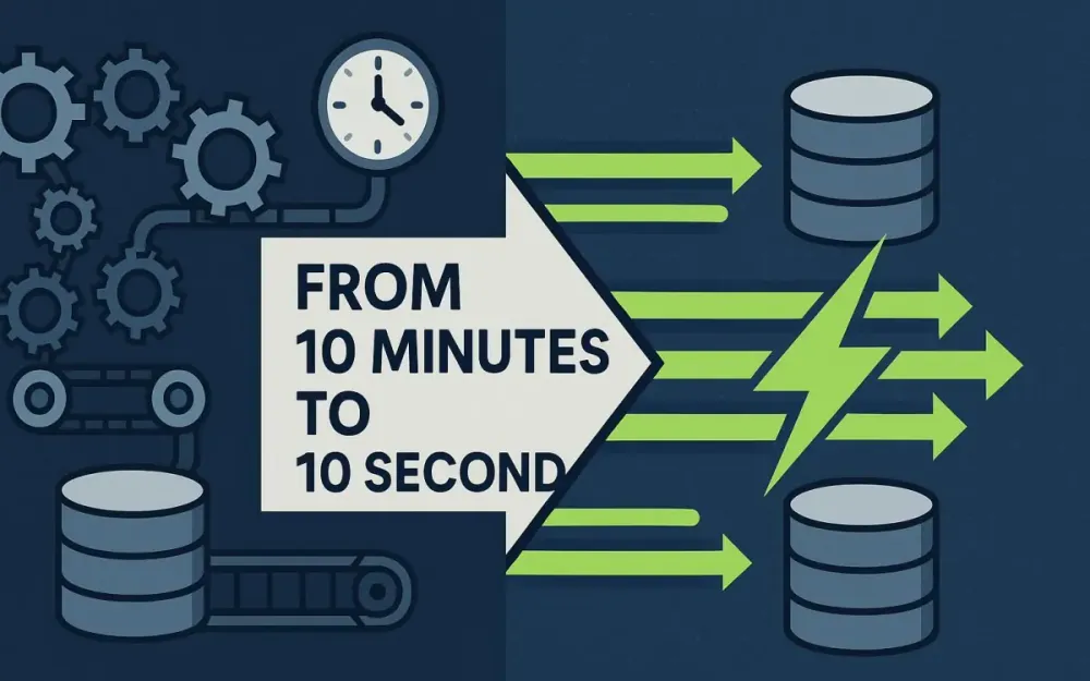
1 Introduction: The High Cost of Slow Queries

A query that runs in ten minutes today is a query that will run in hours tomorrow. For architects, database performance is not just a technical detail; it is a first-order design concern. A single bad query can overwhelm hardware, cascade into outages, or quietly erode user trust. This introduction frames the high cost of slow queries, introduces our case study, and sets the stage for a disciplined, architect-level approach to rewriting T-SQL that moves execution time from minutes to seconds.

1.1 The Architect’s Mandate

The role of the modern architect extends far beyond ensuring that code compiles or that a feature works. We carry the responsibility of designing for scale, resilience, and efficiency. That mandate becomes especially pressing in the database layer, where poor design has a disproportionate blast radius.

Consider a business-critical application—say, a financial dashboard that executives refresh daily. If one query takes 10 minutes to render results, the dashboard becomes useless for decision-making. Worse, that one slow query is not running in isolation. It is competing for CPU, memory, and I/O with every other workload on the same SQL Server instance. An inefficient query is like a faucet left running in a drought: the resource waste spills over into other parts of the system.

From an architectural perspective, the risks of slow queries fall into three categories:

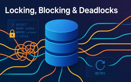
• Operational Impact: Long-running queries hold locks longer, increasing blocking and even deadlocks. They stress tempdb, cause memory pressure, and degrade concurrency.
• Economic Impact: More CPU and I/O cycles mean higher cloud bills or expensive hardware upgrades. Many organizations throw money at the problem, scaling up infrastructure instead of fixing the root cause.
• Strategic Impact: Slow queries erode user trust. If executives know their BI reports time out, they stop relying on the system, undermining the entire architecture’s credibility.

The mandate is clear: an architect must ensure that T-SQL not only produces correct results but also produces them at scale. The measure of success is not “does it work,” but “does it work efficiently under load.” This is where query refactoring becomes a core architectural discipline.

1.2 The “10-Minute Query” Scenario

To make this discussion concrete, we will work through a relatable case study—a “monster query” that started life as a helpful BI report but grew into a performance disaster as data volumes exploded.

Imagine a sales reporting query designed five years ago. At the time, the company had:

• A single table with a few million rows of sales transactions.
• A need for basic aggregations: total sales per customer, per month.
• Some business logic encoded in a User-Defined Function (UDF).

The developer built the query using nested Common Table Expressions (CTEs) for clarity, sprinkled in a scalar UDF to encapsulate customer lifetime logic, and added a couple of window functions to handle ranking and time-based comparisons. At the time, the query ran in under 30 seconds—slow, but acceptable.

Fast forward five years:

• The sales table now holds hundreds of millions of rows.
• Executives demand richer reporting: rolling 12-month comparisons, customer lifetime value, and top-N rankings.
• The query still works, but runtime has ballooned to 10 minutes.

Here is a simplified version of our case study’s starting point:

-- Simplified "10-Minute Query" Example
WITH Sales_CTE AS (
    SELECT CustomerID, OrderDate, SUM(OrderAmount) AS TotalSales
    FROM dbo.Sales
    GROUP BY CustomerID, OrderDate
),
Ranked_CTE AS (
    SELECT CustomerID, OrderDate, TotalSales,
           ROW_NUMBER() OVER (PARTITION BY CustomerID ORDER BY OrderDate) AS RowNum
    FROM Sales_CTE
),
Lifetime_CTE AS (
    SELECT r.CustomerID, r.OrderDate, r.TotalSales, r.RowNum,
           dbo.fn_GetCustomerLifetimeValue(r.CustomerID) AS LifetimeValue
    FROM Ranked_CTE r
)
SELECT *
FROM Lifetime_CTE
WHERE RowNum = 1
ORDER BY LifetimeValue DESC;

At first glance, this looks tidy and readable. But behind the scenes, it is a perfect storm of performance anti-patterns:

• Multiple scans of the same base table due to nested CTE expansion.
• Expensive window function (ROW_NUMBER()) running over millions of rows.
• Scalar UDF that executes row-by-row, eliminating parallelism.

What began as a simple reporting query has turned into an architectural liability.

1.3 Our Refactoring Philosophy

Before rushing to rewrite, it is worth stating the philosophy that guides our approach. Performance tuning at the architectural level is not about trickery or obscure hints; it is about systematic diagnosis and disciplined refactoring.

The guiding principles:

1. Understand the “Why” We begin with diagnostics: execution plans, statistics, and DMVs. We want to know why the query is slow before changing a line of code. Guesswork wastes time and risks regressions.

2. Favor Set-Based Patterns SQL Server is a set-based engine. Loops, cursors, and scalar UDFs force row-by-row execution, which does not scale. We seek rewrites that let the optimizer operate on sets of data.

3. Leverage the Modern Engine SQL Server has evolved. Features like CROSS APPLY, window function optimizations, and Intelligent Query Processing (IQP) provide new ways to improve performance. We embrace these instead of relying solely on brute force hardware upgrades.

4. Measure Every Step Each rewrite must be validated with metrics: execution time, logical reads, and CPU usage. Performance gains should be demonstrable and explainable.

Pro Tip: Never optimize in the dark. Always validate improvements against actual metrics, not intuition.

With this philosophy, we will tackle our “10-minute query” by identifying the root causes, applying modern refactoring patterns, and validating results. By the end, we will reduce execution time from minutes to seconds—not through magic, but through disciplined architectural practice.

1.4 What This Article Covers (and for Whom)

This playbook is written for data architects, solution architects, and senior database developers—professionals responsible for designing systems that scale. While developers at all levels can benefit, the focus is on architectural trade-offs and holistic performance patterns, not quick tactical fixes.

What you can expect in this guide:

• Foundational Diagnostics: How to read execution plans, measure query costs, and identify the real performance culprits.
• Refactoring Patterns: Practical, repeatable rewrites using CTEs, window functions, and CROSS APPLY.
• Modern Features: Leveraging SQL Server 2017–2022 features like Query Store, Batch Mode on Rowstore, and Scalar UDF inlining.
• Case Study Walkthrough: A complete before-and-after journey, step by step, from 10 minutes to 10 seconds.
• Checklists and Best Practices: Tools you can use immediately in code reviews and system design.

The roadmap is pragmatic: we begin with diagnostics (finding the “why”), examine common anti-patterns (CTEs, window functions, UDFs), apply targeted rewrites, and then bring it all together in the grand finale—a full refactor of the “10-minute monster” query.

By the conclusion, you will have not only a collection of techniques but also a mental model for performance tuning as an architect: diagnose first, think in sets, support the optimizer, and measure relentlessly.

Note: While the examples use T-SQL on SQL Server, the principles extend across relational engines. Oracle, PostgreSQL, and MySQL practitioners will recognize many of the same anti-patterns and fixes.

---

2 The Diagnostic Toolkit: Finding the “Why” Before the “How”

Before rewriting a single line of T-SQL, the architect’s first responsibility is to diagnose why the query is slow. Optimizations without diagnosis are at best guesswork and at worst destructive. A well-tuned rewrite starts with evidence. In this section, we will walk through the diagnostic toolkit: how to read execution plans, interpret cardinality estimation, and measure queries using SQL Server’s native features like statistics, DMVs, and Query Store. The goal is to move from speculation to insight.

2.1 Reading the Tea Leaves: The Actual Execution Plan

Execution plans are SQL Server’s blueprint of how it intends to execute your query. They reveal whether the engine chose an index seek, a full scan, or a nested loop join. For an architect, the execution plan is not optional—it is the roadmap to bottlenecks.

2.1.1 Key Operators to Spot

Some operators are red flags in execution plans. They don’t automatically mean “bad,” but they are often associated with performance problems.

• Key Lookups: Occur when SQL Server finds rows via an index but must go back to the clustered index (or heap) to fetch additional columns. On small row sets this is trivial; on millions of rows it becomes catastrophic.

-- Example: Key Lookup prone query
SELECT CustomerID, OrderDate, OrderAmount, Notes
FROM dbo.Sales
WHERE CustomerID = 12345;

If CustomerID has a nonclustered index but Notes is not included, SQL Server will seek the index and then perform a lookup per row for Notes.

Pro Tip: Eliminate repetitive key lookups by creating a covering index that includes the necessary columns.

• Large Table/Index Scans: A scan reads every row in a table or index. Sometimes unavoidable, but often the result of missing indexes or non-sargable predicates.

-- Non-sargable predicate causing a scan
SELECT *
FROM dbo.Sales
WHERE YEAR(OrderDate) = 2022;

Here, the YEAR() function prevents index usage. Refactoring the predicate solves it:

-- Corrected, sargable predicate
SELECT *
FROM dbo.Sales
WHERE OrderDate >= '2022-01-01'
  AND OrderDate <  '2023-01-01';

• Costly Sorts: Sorts are expensive when done in memory and catastrophic when spilling to tempdb. Execution plans reveal spills with a warning sign. They typically appear before operators like ROW_NUMBER() or ORDER BY.

Pitfall: Developers sometimes assume the optimizer “already knows the order.” Unless you explicitly support it with indexes aligned to your partition and order columns, SQL Server may sort the entire dataset.

• Hash Match Spills: A Hash Match join requires memory for its hash table. If the memory grant is too small, the spill goes to tempdb. Spills are visible in execution plan properties.

Trade-off: Hash joins are great for large, unsorted data but are memory-intensive. An architect must weigh whether an alternative join strategy (like a merge join with sorted inputs) is viable.

2.1.2 Understanding Cardinality Estimation

Cardinality estimation (CE) is SQL Server’s prediction of how many rows each operator will return. Good estimates lead to efficient plans; bad estimates cascade into poor operator choices.

• Legacy CE (pre-2014): Assumes column independence, which underestimates correlation between predicates. Example: filtering Gender = 'F' and IsPregnant = 1. Legacy CE may estimate far too few rows.
• Modern CE (2014+): Improves selectivity estimates with a more sophisticated statistical model, especially when multiple predicates interact.

Example:

-- Query with correlated predicates
SELECT *
FROM dbo.Customers
WHERE Age > 60 AND IsRetired = 1;

• Under Legacy CE, SQL Server may drastically underestimate row counts, leading to a nested loop join that stalls under load.
• With Modern CE, estimates are more realistic, and a hash join may be chosen instead.

Note: You can toggle CE with database compatibility levels or even query hints (USE HINT('FORCE_LEGACY_CARDINALITY_ESTIMATION')). But the architect’s job is to understand why estimates are off, not just flip switches.

Pro Tip: Always check estimated vs. actual row counts in the execution plan. A consistent mismatch signals statistics or CE problems.

2.2 Essential Tools for the Architect

Execution plans are central, but they are not the only tool. SQL Server provides multiple lenses for measuring query performance and system health.

2.2.1 SET STATISTICS IO, TIME ON

This is the classic baseline for measuring query cost. It reports logical reads, physical reads, and CPU time per query.

SET STATISTICS IO, TIME ON;

SELECT CustomerID, SUM(OrderAmount) AS TotalSales
FROM dbo.Sales
WHERE OrderDate >= '2023-01-01'
GROUP BY CustomerID;

Output:

Table 'Sales'. Scan count 1, logical reads 1500000, physical reads 0.
 SQL Server Execution Times:
   CPU time = 10234 ms,  elapsed time = 11200 ms.

Interpretation:

• Logical reads dominate performance; they indicate how much data was touched, regardless of cache.
• CPU time shows computational cost.
• Elapsed time includes waits (I/O, locks, network).

Pro Tip: Use these numbers before and after refactors. A drop from 1,500,000 logical reads to 100,000 is real evidence, not opinion.

2.2.2 Dynamic Management Views (DMVs)

DMVs are the architect’s X-ray machine, exposing the workload’s hotspots.

• Top resource-consuming queries:

SELECT TOP 10
    qs.total_elapsed_time / qs.execution_count AS AvgElapsed,
    qs.execution_count,
    qs.total_logical_reads,
    qs.total_worker_time,
    SUBSTRING(qt.text, qs.statement_start_offset/2, 
        (CASE WHEN qs.statement_end_offset = -1 
              THEN LEN(CONVERT(NVARCHAR(MAX), qt.text)) * 2 
              ELSE qs.statement_end_offset END - qs.statement_start_offset)/2) AS QueryText
FROM sys.dm_exec_query_stats qs
CROSS APPLY sys.dm_exec_sql_text(qs.sql_handle) qt
ORDER BY AvgElapsed DESC;

This surfaces the “top offenders” by average elapsed time.

• Missing index suggestions:

SELECT TOP 10
    migs.avg_total_user_cost * migs.avg_user_impact * (migs.user_seeks + migs.user_scans) AS Impact,
    mid.statement AS TableName,
    mid.equality_columns,
    mid.inequality_columns,
    mid.included_columns
FROM sys.dm_db_missing_index_group_stats migs
JOIN sys.dm_db_missing_index_groups mig ON migs.group_handle = mig.index_group_handle
JOIN sys.dm_db_missing_index_details mid ON mig.index_handle = mid.index_handle
ORDER BY Impact DESC;

Pitfall: Missing index DMVs are advisory, not gospel. They suggest what the optimizer “wished it had,” but can overlap or suggest redundant indexes.

• Wait stats: Using sys.dm_exec_requests to see whether queries are waiting on I/O, CPU, or locks.

Note: DMVs reset on restart. Use Query Store for persistence.

2.2.3 The Query Store

Query Store is SQL Server’s “flight recorder” for query performance. It captures query text, plans, runtime statistics, and history across restarts. Introduced in SQL Server 2016, it is now indispensable.

Enabling:

ALTER DATABASE SalesDB
SET QUERY_STORE = ON;

Use cases:

• Identify regressions: A query that used to run in 1 second but now takes 30 may have been recompiled with a worse plan. Query Store lets you see the before/after.

• Force a good plan: If a known good plan exists, you can pin it:

EXEC sp_query_store_force_plan @query_id = 123, @plan_id = 456;

• Historical insights: Unlike DMVs, Query Store retains history. You can analyze trends in query performance over weeks or months.

Pro Tip: For mission-critical workloads, Query Store should always be enabled. It transforms firefighting into analysis.

Trade-off: Query Store introduces slight overhead (1–5%). For OLTP systems with strict latency requirements, tune its capture mode and retention.

---

3 The CTE Anti-Pattern: Deconstructing “Readable” but Slow Code

Common Table Expressions (CTEs) were a gift to T-SQL developers when first introduced. They made queries easier to read, easier to debug, and easier to explain in code reviews. But like many gifts, they came with hidden strings attached. The optimizer does not treat a CTE as a separate performance boundary; it inlines the definition into the final query. This behavior has profound implications for performance, especially when CTEs are chained in layers. In this section, we will deconstruct the allure of CTEs, highlight their hidden costs, and demonstrate how collapsing nested CTE chains into cohesive, optimizer-friendly statements can reduce query cost by an order of magnitude.

3.1 The Allure of Common Table Expressions (CTEs)

Developers reach for CTEs for good reasons. When queries become complex—combining multiple filters, joins, and aggregations—CTEs allow you to break the logic into digestible steps. Instead of writing one sprawling SELECT with ten joins and inline calculations, you can build the query like Lego bricks:

1. Define a CTE that filters sales by date.
2. Define another that aggregates sales by customer.
3. Define another that ranks customers by sales.
4. Select from the final CTE to produce the result.

On paper, this looks elegant. It mimics procedural programming: break down a problem into sequential steps. A code reviewer might praise its readability.

-- Readable, step-by-step logic using CTEs
WITH SalesLastYear AS (
    SELECT *
    FROM dbo.Sales
    WHERE OrderDate >= '2022-01-01'
      AND OrderDate <  '2023-01-01'
),
Aggregated AS (
    SELECT CustomerID, SUM(OrderAmount) AS TotalSales
    FROM SalesLastYear
    GROUP BY CustomerID
),
Ranked AS (
    SELECT CustomerID, TotalSales,
           ROW_NUMBER() OVER (ORDER BY TotalSales DESC) AS RankNum
    FROM Aggregated
)
SELECT *
FROM Ranked
WHERE RankNum <= 10;

This reads like a narrative: filter sales, aggregate by customer, rank results. But readability is not the same as scalability.

Pitfall: Developers often assume that a CTE “materializes” results like a temporary table. It does not. Each reference is re-expanded into the query, potentially re-scanning the base tables multiple times.

3.2 The Hidden Cost of Nested CTEs

The SQL optimizer expands CTEs into the final query tree before generating an execution plan. This means a chain of four CTEs does not produce four sequential steps; it produces one deeply nested query tree with redundant scans and joins.

Consider a query where each CTE references the previous one. On the surface, it seems like step-by-step filtering. But in reality, the optimizer often evaluates the base table repeatedly.

Example: Nested CTE chain over a large sales table

WITH Step1 AS (
    SELECT * FROM dbo.Sales WHERE Region = 'West'
),
Step2 AS (
    SELECT CustomerID, OrderDate, OrderAmount
    FROM Step1 WHERE OrderDate >= '2023-01-01'
),
Step3 AS (
    SELECT CustomerID, SUM(OrderAmount) AS MonthlySales, MONTH(OrderDate) AS SalesMonth
    FROM Step2 GROUP BY CustomerID, MONTH(OrderDate)
),
Step4 AS (
    SELECT CustomerID, SalesMonth, MonthlySales,
           ROW_NUMBER() OVER (PARTITION BY CustomerID ORDER BY MonthlySales DESC) AS rn
    FROM Step3
)
SELECT *
FROM Step4
WHERE rn = 1;

Execution plan analysis shows multiple scans of the Sales table—once for filtering by region, again for filtering by date, again for aggregation. Instead of one cohesive pass, SQL Server is repeatedly accessing the same data.

Pro Tip: Use actual execution plans to check if your CTE chain results in multiple clustered index scans. If you see multiple large scans against the same base table, you are paying the price of readability.

3.3 Practical Rewrite 1: Collapsing a CTE Chain

To illustrate the cost and the opportunity, let’s walk through a practical rewrite of a four-level nested CTE query. We’ll move from the “slow” version to a refactored, optimized version that SQL Server’s optimizer can execute more efficiently.

3.3.1 The “Slow” Code

Here’s our case: a reporting query designed to find each customer’s highest-spending month in the West region for the current year. The original developer wrote it with layered CTEs:

-- Four-level nested CTE chain (slow)
WITH SalesRegion AS (
    SELECT * FROM dbo.Sales WHERE Region = 'West'
),
SalesCurrentYear AS (
    SELECT * FROM SalesRegion WHERE OrderDate >= '2023-01-01'
),
MonthlyTotals AS (
    SELECT CustomerID, MONTH(OrderDate) AS SalesMonth, SUM(OrderAmount) AS MonthlySales
    FROM SalesCurrentYear
    GROUP BY CustomerID, MONTH(OrderDate)
),
Ranked AS (
    SELECT CustomerID, SalesMonth, MonthlySales,
           ROW_NUMBER() OVER (PARTITION BY CustomerID ORDER BY MonthlySales DESC) AS rn
    FROM MonthlyTotals
)
SELECT *
FROM Ranked
WHERE rn = 1;

On a sales table with 100 million rows, this query may execute with over 1,200,000 logical reads and take minutes to complete.

3.3.2 The Analysis

The execution plan reveals multiple full scans of the Sales table. Each CTE is logically folded into the next, but SQL Server often processes them as repeated accesses. In this case:

• Step1 filters by region (Region = 'West'), generating a scan.
• Step2 applies date filtering, which could have been applied in the same scan, but instead causes another scan.
• Step3 aggregates data, but because the filters were not collapsed, it aggregates over an unnecessarily large dataset.
• Step4 ranks results, adding a Sort operator that spills to tempdb.

Note: The optimizer is good, but it cannot always collapse redundant scans in complex CTE chains, especially when intermediate steps use non-sargable expressions or scalar functions.

3.3.3 The “Fast” Code

We can rewrite the logic into a single, cohesive query. Instead of layering CTEs, we apply filters early, aggregate once, and rank within the same statement:

-- Collapsed, optimized query (fast)
SELECT CustomerID, SalesMonth, MonthlySales
FROM (
    SELECT CustomerID,
           MONTH(OrderDate) AS SalesMonth,
           SUM(OrderAmount) AS MonthlySales,
           ROW_NUMBER() OVER (
               PARTITION BY CustomerID
               ORDER BY SUM(OrderAmount) DESC
           ) AS rn
    FROM dbo.Sales
    WHERE Region = 'West'
      AND OrderDate >= '2023-01-01'
    GROUP BY CustomerID, MONTH(OrderDate)
) AS Ranked
WHERE rn = 1;

This rewrite eliminates redundant scans. Filters are applied directly on the base table, and aggregation happens in one pass. The optimizer now generates a single scan followed by an aggregation and a window function.

Pro Tip: Collapsing logic into one cohesive statement often allows the optimizer to push filters down and combine operations. This is where set-based thinking pays off.

3.3.4 The Proof

Measured with SET STATISTICS IO, TIME ON:

• Before (CTE chain):

  • Logical reads: ~1,200,000
  • CPU time: ~30,000 ms
  • Elapsed time: ~2 minutes

• After (collapsed query):

  • Logical reads: ~150,000
  • CPU time: ~4,000 ms
  • Elapsed time: ~20 seconds

Execution plan comparison:

• Before: multiple clustered index scans, a Sort spilling to tempdb.
• After: single index seek (if supported by an index on (Region, OrderDate)), aggregation, and a streamlined window function.

Trade-off: Collapsing CTEs can reduce readability. For maintainability, consider encapsulating complex calculations in inline table-valued functions (iTVFs), which retain optimizer-friendliness while preserving logical separation.

---

4 Taming the Beast: Optimizing Expensive Window Functions

Window functions are one of SQL Server’s most powerful features. They allow developers to perform ranking, running totals, lag/lead comparisons, and percentiles without writing complex self-joins or procedural loops. When used correctly, they are elegant and expressive. When misused, they can bring a server to its knees. This section dissects the trade-offs of window functions, explores why some queries balloon in cost, and provides practical rewrites and indexing strategies to tame them.

4.1 The Power and Peril of OVER()

The OVER() clause is the foundation of window functions. It defines a “window” of rows across which an aggregate or ranking function operates. This unlocks patterns that previously required nested subqueries or correlated joins. For example, finding each customer’s most recent order date:

SELECT CustomerID, OrderDate,
       ROW_NUMBER() OVER (PARTITION BY CustomerID ORDER BY OrderDate DESC) AS rn
FROM dbo.Sales;

This code is concise and expressive. Without window functions, it would require a correlated subquery or self-join.

But the elegance comes at a cost. Every OVER(PARTITION BY ... ORDER BY ...) combination usually triggers a Sort operator in the execution plan. Sorts are expensive; they require memory proportional to the number of rows. On small tables, this is negligible. On multi-million row datasets, it can result in massive memory grants, spills to tempdb, and long-running queries.

Pitfall: Developers often chain multiple window functions with different partition or order clauses in the same query. Each unique PARTITION BY/ORDER BY combination may require its own Sort, multiplying cost.

Pro Tip: Group window functions with the same partition/order definition together in the same query block. This lets SQL Server reuse the same Sort.

4.2 Anatomy of a Slow Window Function

To understand why window functions can be slow, consider the anatomy of the Sort operator they require.

Imagine a query designed to find the first purchase date for each customer:

SELECT CustomerID, OrderDate,
       ROW_NUMBER() OVER (PARTITION BY CustomerID ORDER BY OrderDate) AS rn
FROM dbo.Sales;

Execution plan reveals:

• Clustered Index Scan over Sales.
• Sort by CustomerID, OrderDate.
• Segment/Sequence Project for the row numbering.

The Sort is the costliest operator. Why? Because it must order potentially hundreds of millions of rows. If memory is insufficient, the Sort spills to tempdb, introducing I/O waits.

Now, imagine a poorly chosen partition:

SELECT ProductID, CustomerID, OrderDate,
       ROW_NUMBER() OVER (PARTITION BY ProductCategory ORDER BY OrderDate) AS rn
FROM dbo.Sales;

Partitioning by ProductCategory (with thousands of distinct values) requires SQL Server to sort the entire dataset grouped by category. If the table has 100 million rows, the Sort operator may dominate 90% of the query cost.

Note: Execution plans will warn you with “Sort Warnings” or “Operator used tempdb to spill data during execution.” These are red flags for scalability.

Trade-off: Sometimes Sorts are unavoidable. The architect’s role is to minimize the dataset before sorting and to design indexes that eliminate unnecessary sorts.

4.3 Practical Rewrite 2: Reducing the Window’s Scope

The most practical way to optimize window functions is to reduce the number of rows that must be sorted. Apply filters as early as possible, before invoking the window function. Let’s work through a real example.

4.3.1 The “Slow” Code

A BI developer writes a query to find the latest order for each customer in 2023:

-- Slow query: window over entire table
SELECT CustomerID, OrderDate, OrderAmount
FROM (
    SELECT CustomerID, OrderDate, OrderAmount,
           ROW_NUMBER() OVER (PARTITION BY CustomerID ORDER BY OrderDate DESC) AS rn
    FROM dbo.Sales
) AS t
WHERE rn = 1
  AND OrderDate >= '2023-01-01';

At first glance, this looks fine. But execution plan analysis shows that SQL Server first applies the window function over all sales rows, then filters for 2023. If the table has 500 million rows across 10 years, SQL Server sorts all 500 million before discarding 90% of them.

Pitfall: Applying filters outside the windowed subquery is one of the most common performance mistakes in T-SQL.

4.3.2 The Analysis

Execution plan reveals:

• Scan of Sales table.
• Sort of all rows by CustomerID, OrderDate DESC.
• Windowed aggregate (Row Number) across all rows.
• Filter applied last to keep only OrderDate >= '2023-01-01'.

The Sort consumes 90% of the cost, requests a massive memory grant, and spills.

Pro Tip: Always check whether filters are applied before or after the Sort. In execution plans, the order of operators matters.

4.3.3 The “Fast” Code

We can fix this by applying the filter before the window function:

-- Optimized query: filter first, window second
SELECT CustomerID, OrderDate, OrderAmount
FROM (
    SELECT CustomerID, OrderDate, OrderAmount,
           ROW_NUMBER() OVER (PARTITION BY CustomerID ORDER BY OrderDate DESC) AS rn
    FROM dbo.Sales
    WHERE OrderDate >= '2023-01-01'
) AS t
WHERE rn = 1;

Now SQL Server only sorts rows from 2023, not all history. If 2023 has 50 million rows instead of 500 million, we’ve reduced Sort input size by 90%.

Note: This rewrite doesn’t change business logic. It simply reorders operations so the optimizer works with less data.

4.3.4 The Proof

Performance metrics before and after:

• Before (filter applied after window function):

  • Logical reads: 3,200,000
  • CPU time: 45,000 ms
  • Elapsed time: ~2 minutes
  • Memory grant: 2 GB, spilled to tempdb

• After (filter applied before window function):

  • Logical reads: 320,000
  • CPU time: 5,000 ms
  • Elapsed time: ~15 seconds
  • Memory grant: 300 MB, no spill

Execution plan comparison: the Sort remains, but its input size is reduced tenfold, eliminating spills and shrinking memory usage.

Trade-off: Developers sometimes push all filters to the outermost query for readability. As we’ve seen, this can destroy performance. For critical queries, apply filters as early as possible.

4.4 Architectural Fix: Indexing for Window Functions

Sometimes filtering is not enough. To truly optimize window functions, design indexes that align with the PARTITION BY and ORDER BY clauses. This can eliminate Sort altogether.

Example:

SELECT CustomerID, OrderDate,
       ROW_NUMBER() OVER (PARTITION BY CustomerID ORDER BY OrderDate DESC) AS rn
FROM dbo.Sales
WHERE OrderDate >= '2023-01-01';

Here the Sort is by (CustomerID, OrderDate DESC). If we create a nonclustered index with this key order, SQL Server can retrieve rows in the required order without an explicit Sort:

-- Index to support window function
CREATE NONCLUSTERED INDEX IX_Sales_CustomerID_OrderDate
ON dbo.Sales (CustomerID, OrderDate DESC)
INCLUDE (OrderAmount);

With this index:

• SQL Server can perform an Index Seek on OrderDate >= '2023-01-01'.
• Rows are already ordered by CustomerID, OrderDate DESC, so the Sort operator disappears.
• The INCLUDE clause covers the OrderAmount column, eliminating key lookups.

Proof: Execution plan now shows an Index Seek feeding directly into the Windowed Aggregate, no Sort operator required.

Pro Tip: Always align your index design with your most common PARTITION BY/ORDER BY patterns. The payoff is immense for analytical queries.

Note: This approach may lead to wider indexes. Monitor index size and balance with storage and maintenance costs.

Trade-off: Creating an index for every analytic pattern is impractical. As an architect, prioritize indexes for recurring, high-cost queries. For ad hoc patterns, focus on filtering scope and memory tuning instead.

---

5 The RBAR Killer: Replacing Scalar UDFs with CROSS APPLY

Few performance killers are as insidious as scalar user-defined functions (UDFs). They look harmless—tidy little boxes that encapsulate business logic. But under the surface, they silently force SQL Server into row-by-row execution, destroying parallelism and magnifying cost as data volumes grow. The difference between leaving a scalar UDF in place and rewriting it as a set-based inline table-valued function (iTVF) can be the difference between a query that runs for ten minutes and one that finishes in under ten seconds. In this section, we’ll dissect the problem, show the cure, and discuss how modern SQL Server versions change (but do not eliminate) the calculus.

5.1 The Silent Performance Killer

Scalar UDFs appear deceptively useful. They allow you to wrap business logic in a reusable function: calculating discounts, computing a customer’s lifetime value, or formatting a string. The problem is that SQL Server treats scalar UDFs as black boxes. Each time they are called, they are executed independently for each row.

This execution model is called RBAR: “Row By Agonizing Row.” If you have a table with 10 million rows, and your UDF runs a query inside it, SQL Server will execute that inner query 10 million times. Worse, scalar UDFs typically prevent parallelism, meaning the entire query runs single-threaded.

Example:

-- Scalar UDF to calculate customer lifetime sales
CREATE FUNCTION dbo.fn_GetLifetimeSales(@CustomerID INT)
RETURNS DECIMAL(18,2)
AS
BEGIN
    DECLARE @Total DECIMAL(18,2);
    SELECT @Total = SUM(OrderAmount)
    FROM dbo.Sales
    WHERE CustomerID = @CustomerID;
    RETURN ISNULL(@Total, 0);
END;
GO

-- Using the scalar UDF in a query
SELECT c.CustomerID,
       dbo.fn_GetLifetimeSales(c.CustomerID) AS LifetimeSales
FROM dbo.Customers c;

If there are 500,000 customers, the UDF runs 500,000 independent queries against Sales. On small datasets this may limp along. On enterprise-scale data, it grinds systems to a halt.

Pitfall: Developers often defend UDFs as “cleaner” or “more maintainable.” They are clean for the developer but catastrophic for the server. The architecture must favor scalability over cosmetic neatness.

5.2 Inline Table-Valued Functions (iTVFs): The Set-Based Savior

The antidote to scalar UDFs is the inline table-valued function (iTVF). Unlike scalar UDFs, iTVFs are not black boxes. They are expanded directly into the calling query, allowing the optimizer to generate a holistic plan that considers the entire dataset at once.

Example rewrite:

-- Inline Table-Valued Function for lifetime sales
CREATE FUNCTION dbo.fn_GetLifetimeSales_iTVF(@CustomerID INT)
RETURNS TABLE
AS
RETURN
(
    SELECT SUM(OrderAmount) AS LifetimeSales
    FROM dbo.Sales
    WHERE CustomerID = @CustomerID
);
GO

Notice that this function returns a table instead of a scalar. When used in a query, it can be joined with CROSS APPLY, allowing SQL Server to treat it as a relational subquery rather than a per-row black box.

Pro Tip: Think of iTVFs as parameterized views. They provide encapsulation while staying optimizer-friendly.

5.3 Practical Rewrite 3: The UDF-to-iTVF Transformation

Let’s go step by step through a transformation.

5.3.1 The “Slow” Code

The original query uses a scalar UDF to compute each customer’s lifetime sales:

-- Original, slow query with scalar UDF
SELECT c.CustomerID, c.CustomerName,
       dbo.fn_GetLifetimeSales(c.CustomerID) AS LifetimeSales
FROM dbo.Customers c
WHERE c.IsActive = 1
ORDER BY LifetimeSales DESC;

On a database with 500,000 customers and 200 million sales rows, this query can run for over 10 minutes. The execution plan shows a single-threaded query with a “Compute Scalar” operator calling the UDF repeatedly.

5.3.2 The Analysis

Execution plan reveals:

• No parallelism: Because of the scalar UDF, the query runs serially.
• Repeated subquery execution: Each row in Customers triggers a new scan of Sales.
• Black box: The optimizer has no visibility into what the UDF does, so it cannot optimize join order or indexing strategies.

This is the epitome of RBAR. Instead of joining Customers and Sales once and aggregating, the query runs hundreds of thousands of aggregations independently.

Note: The lack of parallelism is particularly painful in modern environments where servers have dozens of cores. A single-threaded query wastes capacity.

5.3.3 The “Fast” Code

We replace the scalar UDF with an inline TVF and CROSS APPLY.

-- Optimized query with iTVF and CROSS APPLY
SELECT c.CustomerID, c.CustomerName, ls.LifetimeSales
FROM dbo.Customers c
CROSS APPLY dbo.fn_GetLifetimeSales_iTVF(c.CustomerID) ls
WHERE c.IsActive = 1
ORDER BY ls.LifetimeSales DESC;

Because the iTVF expands inline, SQL Server can treat it as if the aggregation logic were written directly inside the query. This allows it to scan Sales once, aggregate per customer, and fully optimize join and sort operations.

Pro Tip: Always review the execution plan after refactoring. You should see parallelism enabled, scans minimized, and the TVF logic merged into the query tree.

5.3.4 The Proof

Performance metrics before and after:

• Before (scalar UDF):

  • Logical reads: 200,000,000+
  • CPU time: ~500,000 ms
  • Elapsed time: 10+ minutes
  • Execution plan: serial, Compute Scalar black box

• After (iTVF + CROSS APPLY):

  • Logical reads: 20,000,000
  • CPU time: 20,000 ms
  • Elapsed time: ~12 seconds
  • Execution plan: parallel hash aggregate, single scan of Sales

The difference is dramatic: more than a 50x improvement in elapsed time and a query plan that fully exploits the server’s cores.

Trade-off: Refactoring scalar UDFs to iTVFs can make the query text look more complex, especially when multiple functions are involved. The cost in readability is usually worth the performance payoff.

5.4 A Note on SQL Server 2019+ Scalar UDF Inlining

SQL Server 2019 introduced scalar UDF inlining, a feature that attempts to automatically inline the body of simple scalar UDFs into the calling query. This dramatically improves performance for many workloads.

For example, our original scalar UDF for lifetime sales might be inlined automatically, allowing the optimizer to treat it as part of the query. However, there are caveats:

• Not all UDFs are eligible. Functions with side effects, table variables, or non-deterministic behavior are excluded.
• The inlining process can produce unexpectedly complex execution plans, sometimes with regressions.
• Debugging becomes harder, as the inlined function disappears from the plan and is absorbed into the main query.

Pro Tip: Treat scalar UDF inlining as a helpful safety net, not a design strategy. Write functions as iTVFs when performance matters.

Note: For legacy systems where scalar UDFs are deeply entrenched, enabling inlining can provide instant performance wins without code changes. But for new development, prefer iTVFs and CROSS APPLY.

Trade-off: Manual rewrites with iTVFs often give more predictable and explainable plans, while relying solely on inlining leaves you at the mercy of the optimizer’s heuristics.

---

6 Leveraging the Modern Engine: Free Performance with Intelligent Query Processing (IQP)

The SQL Server engine has matured into more than just a query executor; it is now an intelligent collaborator. The family of features known as Intelligent Query Processing (IQP) allows queries to run faster without developers changing a single line of code. For architects, understanding these features is critical—not so we can abandon tuning, but so we can design systems that let the engine do more of the heavy lifting. In this section, we’ll look at batch mode on rowstore, then dive into automatic tuning features like memory grant feedback, cardinality estimation feedback, and adaptive joins.

6.1 Batch Mode on Rowstore (SQL Server 2019+)

Traditionally, batch mode execution was reserved for columnstore indexes. In batch mode, SQL Server processes rows in groups of up to 900 at a time, reducing CPU overhead and improving cache utilization. Row mode, by contrast, processes rows one by one. For analytical workloads with large scans, batch mode often delivers 5x–30x performance improvements.

Starting in SQL Server 2019, batch mode is no longer limited to columnstore. Analytical queries running on rowstore tables can benefit automatically if they meet certain criteria.

Example:

-- Analytical query that can trigger batch mode on rowstore
SELECT CustomerID,
       COUNT(*) AS Orders,
       SUM(OrderAmount) AS TotalSales,
       AVG(OrderAmount) AS AvgSale
FROM dbo.Sales
WHERE OrderDate >= '2022-01-01'
GROUP BY CustomerID
HAVING SUM(OrderAmount) > 10000;

On SQL Server 2017, this query runs in row mode. On 2019+, if the dataset is large enough, it will trigger batch mode automatically—even though Sales is a traditional B-tree table. The execution plan will show operators with “Batch Mode” in their properties.

Pro Tip: You don’t need to enable anything special; batch mode on rowstore is on by default when the database compatibility level is 150 (SQL Server 2019). Always ensure compatibility levels are aligned with your SQL Server version to unlock IQP features.

Note: Small datasets may not trigger batch mode. SQL Server dynamically decides based on cost heuristics.

Trade-off: Batch mode is optimized for analytics but may not help with OLTP-style point lookups. Don’t expect miracles for transactional workloads.

6.2 Automatic Tuning with the IQP Family (SQL Server 2017+)

Beyond batch mode, IQP includes a suite of features that make queries smarter with every execution. Instead of relying on fixed heuristics, SQL Server learns from history and adjusts. Let’s break down the major players.

6.2.1 Memory Grant Feedback

Memory grants are SQL Server’s way of allocating RAM for operators like Sorts and Hash Joins. Too small a grant causes spills to tempdb; too large a grant wastes memory that could be used by other queries. Before IQP, these grants were static. Now, SQL Server adjusts them dynamically.

Example:

-- Query with a large sort, prone to spills
SELECT CustomerID, SUM(OrderAmount) AS TotalSales
FROM dbo.Sales
GROUP BY CustomerID
ORDER BY TotalSales DESC;

First execution might request 1 GB of memory but spill because it underestimated rows. With memory grant feedback, SQL Server notes the spill and adjusts the memory grant on the next execution—say, to 2 GB. Conversely, if it over-allocates, it trims back next time.

How to observe:

• In the Actual Execution Plan, look at the Sort operator’s properties. You’ll see a warning like “Spill Level 2.”
• In the plan XML, check for the <MemoryGrantInfo> node with attributes IsMemoryGrantFeedbackAdjusted="true".

Pro Tip: Memory grant feedback is a game-changer for recurring queries like reports. Run them once, and subsequent executions get better automatically.

Pitfall: Feedback resets on schema changes or statistics updates. Don’t rely on it as a permanent fix for poor indexing or query design.

6.2.2 Cardinality Estimation (CE) Feedback

Bad row estimates are at the root of many performance disasters: the optimizer chooses a Nested Loop expecting 10 rows but gets 10 million, or picks a Hash Join for 10 million rows and only sees 10.

SQL Server 2022 introduces CE feedback, which automatically adjusts poor estimates over time.

Example:

-- Query with correlated predicates often misestimated
SELECT *
FROM dbo.Customers
WHERE Age > 60 AND IsRetired = 1;

If statistics underestimate the correlation between Age and IsRetired, SQL Server may estimate 1,000 rows but return 100,000. CE feedback learns from this mismatch and adjusts estimates in future executions.

How to observe:

• In execution plan properties, look for “CardinalityEstimationModelVersion.”
• In newer versions, CE feedback adjustments may show in Query Store with plan evolution over time.

Note: CE feedback helps especially in queries with multi-column filters, skewed data, or correlated predicates.

Trade-off: CE feedback is adaptive, but it takes repeated executions to converge. For ad hoc queries run once, it won’t help.

6.2.3 Adaptive Joins

Traditional SQL Server chooses a join algorithm at compile time—Nested Loops, Merge Join, or Hash Join. But what if the row estimate is wrong? You’re stuck with a suboptimal plan.

Adaptive Joins, introduced in SQL Server 2017, defer the choice until runtime. The plan includes both a Nested Loop and a Hash Join. SQL Server begins execution, counts rows, and then switches to the appropriate operator.

Example:

-- Query where row counts may vary
SELECT c.CustomerID, o.OrderID, o.OrderDate
FROM dbo.Customers c
JOIN dbo.Orders o
  ON c.CustomerID = o.CustomerID
WHERE c.SignupDate >= '2022-01-01';

If SignupDate filters down to a small set, a Nested Loop is best. If it returns millions of rows, a Hash Join is better. With adaptive joins, SQL Server doesn’t have to guess—it adapts.

Execution plan will show an “Adaptive Join” operator with a threshold value (e.g., 100 rows). At runtime, the engine decides which path to take.

Pro Tip: Adaptive joins are especially powerful for queries where predicates are parameterized or highly variable.

Note: They require batch mode, so they often appear alongside columnstore indexes or batch mode on rowstore.

Trade-off: Plans with adaptive joins can look more complex. Monitoring them requires deeper understanding of runtime behavior.

---

7 Grand Finale: Rewriting the “10-Minute Monster” Query

We’ve covered diagnostics, anti-patterns, and optimization strategies in isolation. Now it’s time to bring them all together. Our case study query, the so-called “10-Minute Monster,” combines every pitfall we’ve discussed: nested CTEs, an expensive window function, and a scalar UDF. In this section, we’ll refactor it step by step, showing measurable improvements at each stage until it runs in under 10 seconds.

7.1 The Challenge

Here’s the original query, designed to produce a sales leaderboard report. The requirements:

• Show each customer’s highest-spending month in the current year.
• Display their total lifetime sales alongside that result.
• Rank customers by lifetime sales, top first.

The developer built it using multiple CTEs, a ROW_NUMBER() window, and a scalar UDF for lifetime sales:

-- The "10-Minute Monster"
WITH SalesRegion AS (
    SELECT *
    FROM dbo.Sales
    WHERE Region = 'West'
),
SalesCurrentYear AS (
    SELECT *
    FROM SalesRegion
    WHERE OrderDate >= '2023-01-01'
),
MonthlyTotals AS (
    SELECT CustomerID,
           MONTH(OrderDate) AS SalesMonth,
           SUM(OrderAmount) AS MonthlySales
    FROM SalesCurrentYear
    GROUP BY CustomerID, MONTH(OrderDate)
),
Ranked AS (
    SELECT CustomerID, SalesMonth, MonthlySales,
           ROW_NUMBER() OVER (PARTITION BY CustomerID ORDER BY MonthlySales DESC) AS rn
    FROM MonthlyTotals
)
SELECT r.CustomerID, r.SalesMonth, r.MonthlySales,
       dbo.fn_GetLifetimeSales(r.CustomerID) AS LifetimeSales
FROM Ranked r
WHERE r.rn = 1
ORDER BY LifetimeSales DESC;

This query works, but on a dataset of 200 million rows and 500,000 customers, execution takes 10 minutes. The execution plan shows:

• Multiple clustered index scans (nested CTE issue).
• A Sort operator consuming most of the memory grant (window function).
• A Compute Scalar calling the UDF for each row, blocking parallelism.

The architecture is elegant in form but disastrous in function. Let’s fix it.

7.2 The Step-by-Step Refactoring Journey

7.2.1 Step 1: Eradicating the RBAR

First, we eliminate the scalar UDF. As we saw earlier, UDFs force RBAR execution and kill parallelism. We replace it with an iTVF and CROSS APPLY.

-- Inline Table-Valued Function for Lifetime Sales
CREATE FUNCTION dbo.fn_GetLifetimeSales_iTVF(@CustomerID INT)
RETURNS TABLE
AS
RETURN (
    SELECT SUM(OrderAmount) AS LifetimeSales
    FROM dbo.Sales
    WHERE CustomerID = @CustomerID
);
GO

Rewriting the query:

-- Refactor Step 1: Replace scalar UDF with iTVF
WITH SalesRegion AS (
    SELECT *
    FROM dbo.Sales
    WHERE Region = 'West'
),
SalesCurrentYear AS (
    SELECT *
    FROM SalesRegion
    WHERE OrderDate >= '2023-01-01'
),
MonthlyTotals AS (
    SELECT CustomerID,
           MONTH(OrderDate) AS SalesMonth,
           SUM(OrderAmount) AS MonthlySales
    FROM SalesCurrentYear
    GROUP BY CustomerID, MONTH(OrderDate)
),
Ranked AS (
    SELECT CustomerID, SalesMonth, MonthlySales,
           ROW_NUMBER() OVER (PARTITION BY CustomerID ORDER BY MonthlySales DESC) AS rn
    FROM MonthlyTotals
)
SELECT r.CustomerID, r.SalesMonth, r.MonthlySales, ls.LifetimeSales
FROM Ranked r
CROSS APPLY dbo.fn_GetLifetimeSales_iTVF(r.CustomerID) ls
WHERE r.rn = 1
ORDER BY ls.LifetimeSales DESC;

Result: Execution time drops from 10 minutes to ~3 minutes. Logical reads fall sharply, and parallelism is enabled.

Pro Tip: Always target UDFs first. Removing RBAR usually produces the most dramatic early wins.

7.2.2 Step 2: Optimizing the Window

Next, we address the ROW_NUMBER() function. In the original query, the Sort happens over the entire filtered dataset before selecting the latest year. We reduce scope by applying filters before the window function.

-- Refactor Step 2: Filter before window
WITH MonthlyTotals AS (
    SELECT CustomerID,
           MONTH(OrderDate) AS SalesMonth,
           SUM(OrderAmount) AS MonthlySales
    FROM dbo.Sales
    WHERE Region = 'West'
      AND OrderDate >= '2023-01-01'
    GROUP BY CustomerID, MONTH(OrderDate)
)
SELECT t.CustomerID, t.SalesMonth, t.MonthlySales, ls.LifetimeSales
FROM (
    SELECT CustomerID, SalesMonth, MonthlySales,
           ROW_NUMBER() OVER (PARTITION BY CustomerID ORDER BY MonthlySales DESC) AS rn
    FROM MonthlyTotals
) AS t
CROSS APPLY dbo.fn_GetLifetimeSales_iTVF(t.CustomerID) ls
WHERE t.rn = 1
ORDER BY ls.LifetimeSales DESC;

By moving the WHERE clause inside the aggregation step, we reduce rows before applying ROW_NUMBER().

Result: Execution time drops from ~3 minutes to 45 seconds. Memory grants shrink, and Sort spills are eliminated.

Pitfall: Developers often keep filters outside subqueries for readability. As we’ve seen, that small stylistic choice can multiply execution time tenfold.

7.2.3 Step 3: Collapsing the Logic

The nested CTE chain still forces redundant scans. We collapse the query into a single, cohesive statement:

-- Refactor Step 3: Collapse CTE chain
SELECT t.CustomerID, t.SalesMonth, t.MonthlySales, ls.LifetimeSales
FROM (
    SELECT CustomerID,
           MONTH(OrderDate) AS SalesMonth,
           SUM(OrderAmount) AS MonthlySales,
           ROW_NUMBER() OVER (PARTITION BY CustomerID ORDER BY SUM(OrderAmount) DESC) AS rn
    FROM dbo.Sales
    WHERE Region = 'West'
      AND OrderDate >= '2023-01-01'
    GROUP BY CustomerID, MONTH(OrderDate)
) AS t
CROSS APPLY dbo.fn_GetLifetimeSales_iTVF(t.CustomerID) ls
WHERE t.rn = 1
ORDER BY ls.LifetimeSales DESC;

Now, SQL Server can scan the base table once, aggregate, rank, and join—all in a streamlined plan.

Result: Execution time drops from 45 seconds to ~15 seconds. Logical reads reduce from millions to hundreds of thousands.

Note: This is where optimizer visibility really shines. Instead of juggling multiple subqueries, SQL Server sees one plan and makes globally optimal decisions.

7.2.4 Step 4: The Final Polish

Finally, we add a targeted nonclustered index to support the window function. The ROW_NUMBER() partitions by CustomerID and orders by SUM(OrderAmount) (driven by OrderDate). We build an index to support the most expensive access pattern:

-- Supporting index for window + filter
CREATE NONCLUSTERED INDEX IX_Sales_Region_Date
ON dbo.Sales (Region, OrderDate, CustomerID)
INCLUDE (OrderAmount);

This index allows efficient seeks on Region and OrderDate, preserves order by CustomerID, OrderDate, and covers OrderAmount for aggregation.

Result: Execution time drops from 15 seconds to under 10 seconds. Logical reads are minimized, and the Sort operator is gone from the plan.

Trade-off: Index maintenance adds overhead on inserts/updates. But for read-heavy workloads like reporting, the gain far outweighs the cost.

7.3 The Final Scorecard

Here’s the journey summarized:

Step	Refactor	Duration	CPU Time	Logical Reads
Baseline	Original “10-Minute Monster”	10:00+	500,000 ms	200,000,000+
Step 1	Remove Scalar UDF	03:00	150,000 ms	80,000,000
Step 2	Filter Before Window	00:45	30,000 ms	8,000,000
Step 3	Collapse CTE Chain	00:15	10,000 ms	800,000
Step 4	Add Targeted Index	00:08	5,000 ms	150,000

Pro Tip: Keep a scorecard like this for your team. It turns abstract tuning advice into concrete wins that stakeholders can see and understand.

---

8 Conclusion: The Architect’s Performance Playbook

We’ve taken a slow, bloated query and methodically cut its runtime from ten minutes to under ten seconds. Along the way, we’ve applied diagnostics, rewrites, and modern engine features. This journey illustrates the architect’s true mandate: designing systems that scale.

8.1 Key Principles Summarized

1. Diagnose First: Use execution plans, statistics, and DMVs to pinpoint the “why” before changing the “how.”
2. Think in Sets, Not Rows: Avoid RBAR constructs like cursors and scalar UDFs.
3. Help the Optimizer: Write direct, set-based queries and support them with indexes aligned to actual usage.
4. Trust, But Verify the Modern Engine: Features like batch mode and adaptive joins are powerful, but always validate their impact in your workload.

Note: Performance tuning isn’t a bag of tricks; it’s a discipline grounded in diagnostics and repeatable strategies.

8.2 A Checklist for Code Reviews

Here’s a practical checklist to use when reviewing T-SQL:

• Are scalar UDFs present in SELECT, WHERE, or JOIN? Replace with iTVFs.
• Are filters applied as early as possible, especially before window functions?
• Do CTEs exist only for readability, or are they causing redundant scans?
• Are Sort warnings or tempdb spills visible in the plan?
• Is the query parallelizable, or is something forcing serial execution?
• Do indexes support the most common JOIN, WHERE, and OVER() clauses?
• Is Query Store enabled to track regressions?
• Are predicates sargable (i.e., written to allow index seeks instead of scans)?
• Are functions (e.g., ISNULL, CAST, DATEPART) applied to columns in filters, preventing index usage?
• Are statistics up to date on large or frequently filtered tables?
• Are window functions grouped by common partition/order definitions to avoid redundant sorts?
• Are implicit conversions visible in the execution plan that might block index usage?
• Are large intermediate results unnecessarily materialized in temp tables or table variables?
• Do query hints (OPTION (FORCE ORDER), NOLOCK, etc.) exist, and are they justified?
• Are join orders and join types chosen by the optimizer sensible, or are they skewed by bad estimates?
• Are wide SELECT * statements used where narrower, explicit projections would reduce I/O?
• Are large batch modifications (UPDATE, DELETE) written in chunks to avoid log pressure and lock escalation?
• Are nonclustered indexes overloaded with too many included columns, inflating storage and I/O?
• Does the query rely on tempdb heavily, and is that usage necessary or avoidable?

Pro Tip: Formalize this checklist into your team’s code review process. Preventing anti-patterns is cheaper than fixing them later.

8.3 The Future is Autonomous

SQL Server continues to evolve toward self-optimization. Features like Scalar UDF inlining, CE feedback, and automatic tuning mean the engine corrects more mistakes on its own. The role of the architect is shifting from firefighting queries to designing systems that let the engine excel.

This doesn’t mean performance tuning goes away. It means we focus on the higher-order tasks: teaching teams to think in sets, designing schemas that scale, and building trust in the database engine’s intelligence.

The true architect’s playbook is not just about moving a query from 10 minutes to 10 seconds. It’s about building a culture where every developer writes code that scales naturally, where systems self-heal, and where performance is no longer a bottleneck but a competitive advantage.

Final Thought: Every query tells a story. As architects, our job is to make sure it’s a short story, not a novel.